Road to Deep Learning - Part 3: Deep Neural Network and Multi-class classifier
23 Aug 2019
Reading time ~38 minutes
Deep Neural Network
This notebook covers the basics of deep neural networks and their implementation in Python. In Part 1 of this series, we went over the logistic regression. In Part 2, we covered the basis of Neural Networks and their implementation.
Neural Networks were created in an intent to mimic the human vision and the brain structure. Instead of having the entire information process by a neuron, it is process by an network of neurons. Each neuron serves a basic function (detect curves, detect straight lines…) then the information is conveyed to another layer in charge of detecting more complex patter.
Table of Content
1. Notation
2. Theory
3. Implementation in Python
4. Application on MNIST
5. Implementation using Keras
6. Softmax Regression
7. Application of Multiclass on MNIST
8. Conclusion
# load libraries
import numpy as np
import pandas as pd

# personal tools
import TAD_tools_v00

# data generator and data manipulation
from sklearn.datasets import make_classification, make_blobs, make_moons, make_circles, make_classification
from sklearn.model_selection import train_test_split
from sklearn.metrics import accuracy_score, confusion_matrix

# plotting tools
import matplotlib.pyplot as plt
import seaborn as sns
plt.style.use('ggplot')
%matplotlib inline
1. Notations
The following notations are used in this notebook:
- \(m\) is the number of feature of the input
- Type: integer
- \(n\) is the number of input examples
- Type: integer
- \(x\) is the set of input data
- Type: Array
- Size: \((m*n)\)
- Components: \(x^{(i)}\) of size \((m*1)\)
- \(n^{[l]}\) is the number of neurons in the hidden layer (l)
- Type: integer
- \(W^{[l]}\) are the weights of the layer l (hidden)
- Type: Array
- Size: \((n^{[l]}*n^{[l-1]})\)
- \(W^{[L]}\) are the weights of the layer L (output)
- Type: Array
- Size: \((1*n^{[L-1]})\)
- \(b^{[l]}\) are the bias of the layer l (hidden)
- Type: Array
- Size: \((n^{[1]}*1)\)
- \(b^{[L]}\) are the bias of the layer L (output)
- Type: Array
- Size: \((1*1)\)
- \(a^{[l]}\) is the output of the l-th layer
- Type: Array
- Size: \((n^{[l]}*n)\)
- Components: \(a^{[l] (i)}\)
2. Theory
2.1. Components
The deep neural network model is made of the following components:
- The input layer (i.e. the input data)
- Several hidden layers (main difference with simple neural networks)
- One output layer
Each hidden layer (\(l\)) is made of an ensemble of neurons each equipped with the following two tools:
- A set of weights \(\{w_{1}^{[l]},..,w_{m}^{[l]}\}\) and a bias term \(b^{[l]}\).
- An activation function which adds a non-linear behavior to its neuron.
2.2. Architecture
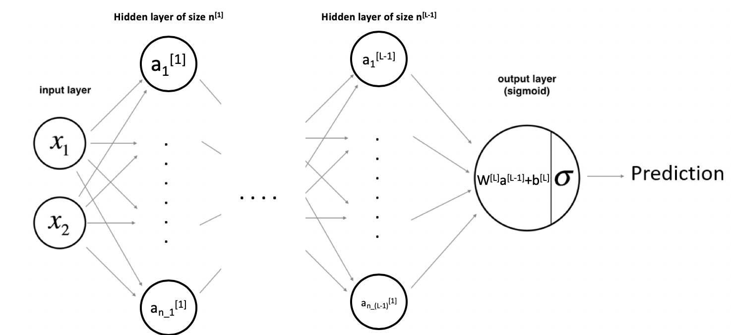
As shown above, the input vector \(X=\{x_{1},x_{2}\}\) passes through the first hidden layer. The output of the hidden layer are then used as an input for the output layer. Finally, the output of the last layer is used to make a prediction.
Let’s take an example where the hidden layer is made of 2 hidden units. The equations of the model are:
\(a_{1}^{[1]}=g(w_{1,1}^{[1]}*x_{1}+w_{1,2}^{[1]}*x_{2}+b_{1}^{[1]})\)
\(a_{2}^{[1]}=g(w_{2,1}^{[1]}*x_{1}+w_{2,2}^{[1]}*x_{2}+b_{2}^{[1]})\)
Then:
\(y_{prob}=\sigma(w_{1}^{[2]}*a_{1}^{[1]}+w_{2}^{[2]}*a_{2}^{[1]}+b^{[2]})\)
2.3. Activation Functions
The activation of the output layer is the sigmoid. This choice is based on the nature of the output, the output layer gives a probability (between 0 and 1). However, the activation layer of the hidden units can be chosen amongst a larger set of functions:
- tanh
- ReLU (Rectified Linear Unit)
- Leaky RelU
- Step
- Linear
# Define the range for plot
x = np.linspace(-2,2,100)

# Define activation functions over range
f_tanh = np.tanh(x)
f_relu = np.maximum(x,0)
f_leaky_relu = np.maximum(x,0.01*x)
f_step = x / 2 / np.abs(x) + 1/2
f_linear = x
# Plot activation functions
fig, axs = plt.subplots(1,2,figsize=(16,6))
axs[0].plot(x, f_tanh, label='tanh', linestyle='-.')
axs[0].plot(x, f_step, label='step')
axs[0].plot(x, f_linear, label='linear', color='orchid', linestyle='--')
axs[1].plot(x, f_relu, label='ReLU: max(x, 0)')
axs[1].plot(x, f_leaky_relu, label='Leaky ReLU: max(x, 0.01*x)', linestyle='--')
axs[0].legend()
axs[1].legend()
fig.suptitle('Activation Functions');
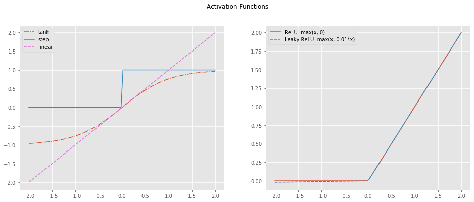
NOTE: For the rest of this post, the tanh function is used. It performs relatively well as it creates the non-linearity needed while spanning between -1 and 1. Small values helps with the optimization.
2.4. Cost Function
Finally, we define the Cost Function as the average of the Loss Function over the entire set of examples.
\[J = \frac{1}{m} \sum_{i=1}^m L(a^{(i)}, y^{(i)})\]The Loss Function for a single example is defined as:
\[L(a^{(i)}, y^{(i)})=- (y^{(i)}\log\left(a^{(i)}\right) - (1-y^{(i)})\log\left(1- a^{(i)}\right))\]2.5. Optimization
Similarly to the simple neural network and the logistic regression, a gradient descent is performed to optimize the various weights of the network. The optimization is performed as a three-step process:
- Forward propagation: Compute the predictions and the various outputs of each layer.
- Backward propagation: Use the results from the previous step to compute the partial derivative of the cost function with respect to each weight.
- Update the weights
Below are the formulas used to compute the gradients.
\(dZ^{[l]} = dA^{[l]} * g'(Z^{[l]})\)
\(dW^{[l]} = \frac{\partial L }{\partial W^{[l]}} = \frac{1}{m} dZ^{[l]} A^{[l-1] T}\)
\(db^{[l]} = \frac{\partial L }{\partial b^{[l]}} = \frac{1}{m} \sum_{i = 1}^{m} dZ^{[l](i)}\)
\(dA^{[l-1]} = \frac{\partial L }{\partial A^{[l-1]}} = W^{[l] T} dZ^{[l]}\)
\(g(.)\) is the activation function
- Note that \(*\) denotes element-wise multiplication.
- The notation you will use is common in deep learning coding:
- dW1 = \(\frac{\partial J }{ \partial W_1 }\)
- db1 = \(\frac{\partial J }{ \partial b_1 }\)
- dW2 = \(\frac{\partial J }{ \partial W_2 }\)
- db2 = \(\frac{\partial J }{ \partial b_2 }\)
3. Implementation in Python
The functions below are used to define the neural network model. They are defined as follows:
- Initialization
a.initialize_parameters_deep: Establish the architecture of the model - Forward Propagation
a.linear_forward: Compute linear activation of the current layer
i.sigmoid: Compute sigmoid of layer output
ii.relu: Compute relu of layer output
b.linear_activation_forward: Compute linear forward and activation function for the current layer
c.L_model_forward: Compute full-forward propagation
d.compute_cost: Compute cost - Backward Propagation
a.linear_backward: Compute partial derivative associated to the linear activation of the current layer
i.relu_backward: Compute partial derivative associated to the relu activation
ii.sigmoid_backward: Compute partial derivative associated to the sigmoid activation
b.linear_activation_backward: Compute partial derivative associated to the current layer
c.L_model_backward: Compute partial derivative associated to the entire model
d.update_parameters: Update all the parameters of the network - Build Model
a.L_layer_model: Build a L-layer deep-neural network
The initialization is kept simple. The weights associated to each neurons are initialized randomly and the bias terms set to 0.
def initialize_parameters_deep(layer_dims):
    """
    Arguments:
    layer_dims -- python array (list) containing the dimensions of each layer in our network

    Returns:
    parameters -- python dictionary containing your parameters "W1", "b1", ..., "WL", "bL":
                    Wl -- weight matrix of shape (layer_dims[l], layer_dims[l-1])
                    bl -- bias vector of shape (layer_dims[l], 1)
    """

    np.random.seed(3)
    parameters = {}                # used to store Wl and bl
    L = len(layer_dims)            # number of layers in the network

    for l in range(1, L):

        # Initialize weights and bias
        parameters['W' + str(l)] = np.random.randn(layer_dims[l],layer_dims[l-1])*0.01
        parameters['b' + str(l)] = np.zeros((layer_dims[l],1))

        assert(parameters['W' + str(l)].shape == (layer_dims[l], layer_dims[l-1]))
        assert(parameters['b' + str(l)].shape == (layer_dims[l], 1))

    return parameters
Two activation functions will be used for this case:
- Relu: used as the activation function of each hidden layer.
- Sigmoid: used as the activation of the output layer.
def sigmoid(Z):
    """
    Implements the sigmoid activation in numpy

    Arguments:
    Z -- numpy array of any shape

    Returns:
    A -- output of sigmoid(z), same shape as Z
    cache -- returns Z as well, useful during back-propagation
    """

    A = 1/(1+np.exp(-Z))
    cache = Z

    return A, cache

def relu(Z):
    """
    Implement the RELU function.

    Arguments:
    Z -- Output of the linear layer, of any shape

    Returns:
    A -- Post-activation parameter, of the same shape as Z
    cache -- a python dictionary containing "A" ; stored for computing the backward pass efficiently
    """

    A = np.maximum(0,Z)

    assert(A.shape == Z.shape)

    cache = Z
    return A, cache
Once the model has been initialized, it is necessary to compute the results of the forward pass. To do so, two functions will be used:
linear_forward: computation of \(Z^{[l]}=W^{[l]}*A^{[l-1]}+b^{[l]}\)linear_activation_forward: computation of \(A^{[l]}=g(Z^{[l]})\)
def linear_forward(A, W, b):
    """
    Implement the linear part of a layer's forward propagation.

    Arguments:
    A -- activations from previous layer (or input data): (size of previous layer, number of examples)
    W -- weights matrix: numpy array of shape (size of current layer, size of previous layer)
    b -- bias vector, numpy array of shape (size of the current layer, 1)

    Returns:
    Z -- the input of the activation function, also called pre-activation parameter
    cache -- a python dictionary containing "A", "W" and "b" ; stored for computing the backward pass efficiently
    """

    Z = np.dot(W,A) + b

    assert(Z.shape == (W.shape[0], A.shape[1]))
    cache = (A, W, b)

    return Z, cache
def linear_activation_forward(A_prev, W, b, activation):
    """
    Implement the forward propagation for the LINEAR->ACTIVATION layer

    Arguments:
    A_prev -- activations from previous layer (or input data): (size of previous layer, number of examples)
    W -- weights matrix: numpy array of shape (size of current layer, size of previous layer)
    b -- bias vector, numpy array of shape (size of the current layer, 1)
    activation -- the activation to be used in this layer, stored as a text string: "sigmoid" or "relu"

    Returns:
    A -- the output of the activation function, also called the post-activation value
    cache -- a python dictionary containing "linear_cache" and "activation_cache";
             stored for computing the backward pass efficiently
    """

    if activation == "sigmoid":
        # Inputs: "A_prev, W, b". Outputs: "A, activation_cache".
        Z, linear_cache = linear_forward(A_prev, W, b)
        A, activation_cache = sigmoid(Z)

    elif activation == "relu":
        # Inputs: "A_prev, W, b". Outputs: "A, activation_cache".
        Z, linear_cache = linear_forward(A_prev, W, b)
        A, activation_cache = relu(Z)

    assert (A.shape == (W.shape[0], A_prev.shape[1]))
    cache = (linear_cache, activation_cache)

    return A, cache
Using the two tool functions defined above to perform the forward propagation through an individual layer, a new function is created to perform the full forward propagation from the input layer to the output layer.
def L_model_forward(X, parameters):
    """
    Implement forward propagation for the [LINEAR->RELU]*(L-1)->LINEAR->SIGMOID computation

    Arguments:
    X -- data, numpy array of shape (input size, number of examples)
    parameters -- output of initialize_parameters_deep()

    Returns:
    AL -- last post-activation value
    caches -- list of caches containing:
                every cache of linear_activation_forward() (there are L-1 of them, indexed from 0 to L-1)
    """

    caches = []
    A = X
    L = len(parameters) // 2                  # number of layers in the neural network

    # Implement [LINEAR -> RELU]*(L-1). Add "cache" to the "caches" list.
    for l in range(1, L):
        A_prev = A

        # retrieve parameters
        W = parameters['W' + str(l)]
        b = parameters['b' + str(l)]
        activation = 'relu'

        A, cache = linear_activation_forward(A_prev, W, b, activation)
        caches.append(cache)

    # Implement LINEAR -> SIGMOID. Add "cache" to the "caches" list.

    # retrieve parameters
    W = parameters['W' + str(L)]
    b = parameters['b' + str(L)]
    activation = 'sigmoid'

    AL, cache = linear_activation_forward(A, W, b, activation)
    caches.append(cache)

    assert(AL.shape == (1,X.shape[1]))

    return AL, caches
The final step before performing the backward propagation consists of computing the cost associated to the forward propagation.
def compute_cost(AL, Y):
    """
    Implement the cost function.

    Arguments:
    AL -- probability vector corresponding to your label predictions, shape (1, number of examples)
    Y -- true "label" vector (for example: containing 0 or 1), shape (1, number of examples)

    Returns:
    cost -- cross-entropy cost
    """

    m = Y.shape[1]

    # Compute loss from aL and y.
    cost = (-1/m) * np.sum( np.log(AL) * Y + np.log(1-AL) * (1 - Y) )

    cost = np.squeeze(cost)      # To make sure your cost's shape is what we expect (e.g. this turns [[17]] into 17).
    assert(cost.shape == ())

    return cost
Now, all the components needed to compute the different partial derivatives associated to the gradient descent are ready. Similarly to the forward propagation, we use a set of tool functions to compute the intermediate calculations associated to the backward propagation:
linear_backward: compute \(dA^{[l]}\) using \(dZ^{[l+1]}\)relu_backward: compute \(dZ^{[l]}\) using \(dA^{[l]}\) for the hidden layerssigmoid_backward: compute \(dZ^{[l]}\) using \(dA^{[l]}\) for the output layer
def linear_backward(dZ, cache):
    """
    Implement the linear portion of backward propagation for a single layer (layer l)

    Arguments:
    dZ -- Gradient of the cost with respect to the linear output (of current layer l)
    cache -- tuple of values (A_prev, W, b) coming from the forward propagation in the current layer

    Returns:
    dA_prev -- Gradient of the cost with respect to the activation (of the previous layer l-1), same shape as A_prev
    dW -- Gradient of the cost with respect to W (current layer l), same shape as W
    db -- Gradient of the cost with respect to b (current layer l), same shape as b
    """
    A_prev, W, b = cache
    m = A_prev.shape[1]

    dW = (1./m) * np.dot(dZ, A_prev.T)
    db = (1./m) * np.sum(dZ,axis=1,keepdims=True)
    dA_prev = np.dot(W.T, dZ)

    assert (dA_prev.shape == A_prev.shape)
    assert (dW.shape == W.shape)
    assert (db.shape == b.shape)

    return dA_prev, dW, db
def relu_backward(dA, cache):
    """
    Implement the backward propagation for a single RELU unit.

    Arguments:
    dA -- post-activation gradient, of any shape
    cache -- 'Z' where we store for computing backward propagation efficiently

    Returns:
    dZ -- Gradient of the cost with respect to Z
    """

    Z = cache
    dZ = np.array(dA, copy=True) # just converting dz to a correct object.

    # When z <= 0, you should set dz to 0 as well.
    dZ[Z <= 0] = 0

    assert (dZ.shape == Z.shape)

    return dZ

def sigmoid_backward(dA, cache):
    """
    Implement the backward propagation for a single SIGMOID unit.

    Arguments:
    dA -- post-activation gradient, of any shape
    cache -- 'Z' where we store for computing backward propagation efficiently

    Returns:
    dZ -- Gradient of the cost with respect to Z
    """

    Z = cache

    s = 1/(1+np.exp(-Z))
    dZ = dA * s * (1-s)

    assert (dZ.shape == Z.shape)

    return dZ
The above functions are combined into a single one. This new functions takes \(dA^{[l+1]}\) as an input and returns \(dA^{[l]}\).
def linear_activation_backward(dA, cache, activation):
    """
    Implement the backward propagation for the LINEAR->ACTIVATION layer.

    Arguments:
    dA -- post-activation gradient for current layer l
    cache -- tuple of values (linear_cache, activation_cache) we store for computing backward propagation efficiently
    activation -- the activation to be used in this layer, stored as a text string: "sigmoid" or "relu"

    Returns:
    dA_prev -- Gradient of the cost with respect to the activation (of the previous layer l-1), same shape as A_prev
    dW -- Gradient of the cost with respect to W (current layer l), same shape as W
    db -- Gradient of the cost with respect to b (current layer l), same shape as b
    """
    # retrieve caches
    # linear_cache = (A, W, b)
    # activation_cache = Z

    linear_cache, activation_cache = cache

    if activation == "relu":

        # parameters
        Z = activation_cache

        dZ = relu_backward(dA, activation_cache)
        dA_prev, dW, db = linear_backward(dZ, linear_cache)

    elif activation == "sigmoid":

        # parameters
        Z = activation_cache

        dZ = sigmoid_backward(dA, activation_cache)
        dA_prev, dW, db = linear_backward(dZ, linear_cache)

    return dA_prev, dW, db
Using the tool functions defined above to perform the backward propagation through an individual layer, a new function is created to perform the full backward propagation from the output layer to the input layer.
def L_model_backward(AL, Y, caches):
    """
    Implement the backward propagation for the [LINEAR->RELU] * (L-1) -> LINEAR -> SIGMOID group

    Arguments:
    AL -- probability vector, output of the forward propagation (L_model_forward())
    Y -- true "label" vector (containing 0 or 1)
    caches -- list of caches containing:
                every cache of linear_activation_forward() with "relu" (it's caches[l], for l in range(L-1) i.e l = 0...L-2)
                the cache of linear_activation_forward() with "sigmoid" (it's caches[L-1])

                for every cache, a tuple is used to store: (linear_cache, activation_cache)
                    linear_cache = (A, W, b)
                    activation_cache = Z

    Returns:
    grads -- A dictionary with the gradients
             grads["dA" + str(l)] = ...
             grads["dW" + str(l)] = ...
             grads["db" + str(l)] = ...
    """
    grads = {}
    L = len(caches) # the number of layers
    m = AL.shape[1]
    Y = Y.reshape(AL.shape) # after this line, Y is the same shape as AL

    # Initializing the backpropagation
    dAL = - (np.divide(Y, AL) - np.divide(1 - Y, 1 - AL))

    # Lth layer (SIGMOID -> LINEAR) gradients. Inputs: "dAL, current_cache". Outputs: "grads["dAL-1"], grads["dWL"], grads["dbL"]
    current_cache = caches[-1]
    grads["dA" + str(L-1)], grads["dW" + str(L)], grads["db" + str(L)] = linear_activation_backward(dAL, current_cache, 'sigmoid')

    # Loop from l=L-2 to l=0
    for l in reversed(range(L-1)):
        # lth layer: (RELU -> LINEAR) gradients.
        # Inputs: "grads["dA" + str(l + 1)], current_cache". Outputs: "grads["dA" + str(l)] , grads["dW" + str(l + 1)] , grads["db" + str(l + 1)]
        current_cache = caches[l]
        dA_prev_temp, dW_temp, db_temp = linear_activation_backward(grads["dA" + str(l+1)], current_cache, 'relu')
        grads["dA" + str(l)] = dA_prev_temp
        grads["dW" + str(l + 1)] = dW_temp
        grads["db" + str(l + 1)] = db_temp

    return grads
Using the various partial derivative terms computed during the backward propagation, the weights and bias are updated.
def update_parameters(parameters, grads, learning_rate):
    """
    Update parameters using gradient descent

    Arguments:
    parameters -- python dictionary containing your parameters
    grads -- python dictionary containing your gradients, output of L_model_backward

    Returns:
    parameters -- python dictionary containing your updated parameters
                  parameters["W" + str(l)] = ...
                  parameters["b" + str(l)] = ...
    """

    L = len(parameters) // 2 # number of layers in the neural network

    # Update rule for each parameter. Use a for loop.
    for l in range(L):
        parameters["W" + str(l+1)] = parameters["W" + str(l+1)] - learning_rate * grads["dW" + str(l+1)]
        parameters["b" + str(l+1)] = parameters["b" + str(l+1)] - learning_rate * grads["db" + str(l+1)]

    return parameters
def L_layer_model(X, Y, layers_dims, learning_rate = 0.075, num_iterations = 3000, print_cost=False):
    """
    Implements a L-layer neural network: [LINEAR->RELU]*(L-1)->LINEAR->SIGMOID.

    Arguments:
    X -- data, numpy array of shape (number of examples, num_px * num_px * 3)
    Y -- true "label" vector (containing 0 or 1), of shape (1, number of examples)
    layers_dims -- list containing the input size and each layer size, of length (number of layers + 1).
    learning_rate -- learning rate of the gradient descent update rule
    num_iterations -- number of iterations of the optimization loop
    print_cost -- if True, it prints the cost every 100 steps

    Returns:
    parameters -- parameters learned by the model. They can then be used to predict.
    """

    np.random.seed(1)
    costs = []                         # keep track of cost

    # Parameters initialization. (≈ 1 line of code)
    parameters = initialize_parameters_deep(layers_dims)

    # Loop (gradient descent)
    for i in range(0, num_iterations):

        # Forward propagation: [LINEAR -> RELU]*(L-1) -> LINEAR -> SIGMOID.
        AL, caches = L_model_forward(X, parameters)

        # Compute cost.
        cost = compute_cost(AL, Y)

        # Backward propagation.
        grads = L_model_backward(AL, Y, caches)

        # Update parameters.
        parameters = update_parameters(parameters, grads, learning_rate)

        # Print the cost every 100 training example
        if print_cost and i % 100 == 0:
            print ("Cost after iteration %i: %f" %(i, cost))
        if print_cost and i % 100 == 0:
            costs.append(cost)

    # plot the cost
    if print_cost:
        print(np.squeeze(costs))
        plt.plot(np.squeeze(costs))
        plt.ylabel('cost')
        plt.xlabel('iterations (per tens)')
        plt.title("Learning rate =" + str(learning_rate))
        plt.show()

    return parameters
def predict(X, y, parameters):
    """
    This function is used to predict the results of a  L-layer neural network.

    Arguments:
    X -- data set of examples you would like to label
    parameters -- parameters of the trained model

    Returns:
    p -- predictions for the given dataset X
    """

    m = X.shape[1]
    n = len(parameters) // 2 # number of layers in the neural network
    p = np.zeros((1,m))

    # Forward propagation
    probas, caches = L_model_forward(X, parameters)

    # convert probas to 0/1 predictions
    for i in range(0, probas.shape[1]):
        if probas[0,i] > 0.5:
            p[0,i] = 1
        else:
            p[0,i] = 0

    #print results
    print("   Accuracy: {:.2f}%%".format(np.sum((p == y)/m)*100))

    return p
4. Application on MNIST
4.1. Data Import
We have defined the necessary tools to build a Deep Neural Network. We will now test our implementation using the famous MNIST dataset. This dataset consists of a set of hand-written digits (0 to 9). Since our model was kept simple and is used to perform binary classification, we will adjust the problem of the digit recognition to detect the digit 5.
import tensorflow as tf
import matplotlib.pyplot as plt
import numpy as np
# load data
mnist = tf.keras.datasets.mnist

(X_train, Y_train), (X_test, Y_test) = mnist.load_data()
print('The shape of the training set is:', X_train.shape)
print('The shape of the training target is:', Y_train.shape)

print('The shape of the test set is:', X_test.shape)
print('The shape of the test target is:', Y_test.shape)
The shape of the training set is: (60000, 28, 28)
The shape of the training target is: (60000,)
The shape of the test set is: (10000, 28, 28)
The shape of the test target is: (10000,)
Before generating our model, we inspect the dataset by potting a few examples for each class.
# unique classes
unique_classes = np.unique(Y_train)

# create plot figure
fig, axes = plt.subplots(10,10,figsize=(9,9))

# loop over the classes and plots a few randomly selected images
for idx, digit in enumerate(unique_classes):
    selected_images = X_train[Y_train==digit][0:10]

    for k in range(0,10):
        axes[digit,k].imshow(selected_images[k],cmap='gray')
        axes[digit,k].axis('off')
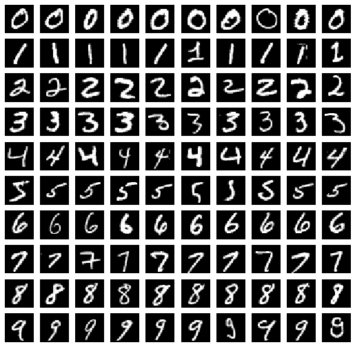
We now extract all the 5 and a random subset of non-five. We want to keep the dataset balance between the two classes (5 and non-5).
np.random.seed(42)

X_train_five = X_train[Y_train==5]
X_train_non_five = X_train[Y_train!=5]
np.random.shuffle(X_train_non_five)
X_train_non_five = X_train_non_five[0:X_train_five.shape[0],:]

Y_train = np.zeros((X_train_five.shape[0]+X_train_non_five.shape[0],), dtype=float)
Y_train[0:X_train_five.shape[0]] = 1

X_test_five = X_test[Y_test==5]
X_test_non_five = X_test[Y_test!=5]
np.random.shuffle(X_test_non_five)
X_test_non_five = X_test_non_five[0:X_test_five.shape[0],:]

Y_test = np.zeros((X_test_five.shape[0]+X_test_non_five.shape[0],), dtype=float)
Y_test[0:X_test_five.shape[0]] = 1

print('There are {} instances of 5 in the train set.'.format(X_train_five.shape[0]))
print('There are {} instances of 5 in the test set.'.format(X_test_five.shape[0]))
There are 5421 instances of 5 in the train set.
There are 892 instances of 5 in the test set.
Finally, we reshape the datasets and scale the pixel values.
# stack classes
X_train = np.vstack([X_train_five, X_train_non_five])
X_test = np.vstack([X_test_five, X_test_non_five])
# reshape
X_train = X_train.reshape(-1,28*28).T
X_test = X_test.reshape(-1,28*28).T

Y_train = Y_train.reshape(1,-1)
Y_test = Y_test.reshape(1,-1)
# normalize
X_train = X_train / 255.0
X_test = X_test / 255.0
print('The shape of the training set is:', X_train.shape)
print('The shape of the training target is:', Y_train.shape)

print('The shape of the test set is:', X_test.shape)
print('The shape of the test target is:', Y_test.shape)
The shape of the training set is: (784, 10842)
The shape of the training target is: (1, 10842)
The shape of the test set is: (784, 1784)
The shape of the test target is: (1, 1784)
4.2. Model Testing
One of the first steps of building a DNN is to define its architecture. That is, the number of hidden layers and the number of hidden units per hidden layers. Various candidates are generated and trained. The best one is kept.
models = {
    '28x28->1':[28*28, 1],
    '28x28->5->1':[28*28, 5, 1],
    '28x28->7->5->1':[28*28, 7, 5, 1],
}
scores = {}

for name, layers_dims in models.items():

    # generate model
    parameters = L_layer_model(X_train, Y_train, layers_dims, num_iterations = 2500, print_cost = False)

    # print name
    print(name)

    # make predictions on train set
    print('Train set:')
    pred_train = predict(X_train, Y_train, parameters)

    # make predictions on test set
    print('Test set:')
    pred_test = predict(X_test, Y_test, parameters)
28x28->1
Train set:
   Accuracy: 92.58%%
Test set:
   Accuracy: 92.60%%
28x28->5->1
Train set:
   Accuracy: 97.35%%
Test set:
   Accuracy: 96.92%%
28x28->7->5->1
Train set:
   Accuracy: 93.17%%
Test set:
   Accuracy: 93.11%%
The 5->1 network gives the best results on the test set. The next phase would consists of tuning the learning rate for this selected architecture.
5. Implementation using Keras
This full implementation of a deep neural network required took time. Luckily, there are now pre-built libraries to help speed up the process. In this next section, we will use Keras.
import tensorflow as tf
from tensorflow.keras.models import Sequential
from tensorflow.keras.layers import Dense
from tensorflow.keras.optimizers import Adam
We re-use the architecture 28x28->5->1.
model = Sequential()
model.add(Dense(128, input_dim=28*28, activation='relu'))
model.add(Dense(5, activation='relu'))
model.add(Dense(1, activation='sigmoid'))
The optimization performed during the gradient descent will be performed using the efficient adam optimizer. The Adam Optimizer uses a exponential average and some scaling to improve the parameter updates and converge quickly toward the best set of parameters.
adam = Adam(lr=0.001)
model.compile(loss='binary_crossentropy', optimizer=adam, metrics=['accuracy'])
In our implementation of the DNN, we implemented the gradient descent using the Batch approach (i.e. the entire training set is processed then the parameters are updated). For this example, we will use a Mini Batch approach were a fraction of the training set is process before the parameters are updated. This choice help improve the results. In this case, 128 training examples are used before each update.
model.fit(X_train.T, Y_train.T, epochs=10, batch_size=128)
Train on 10842 samples
Epoch 1/10
10842/10842 [==============================] - 0s 29us/sample - loss: 0.1973 - accuracy: 0.9257
Epoch 2/10
10842/10842 [==============================] - 0s 13us/sample - loss: 0.0763 - accuracy: 0.9747
Epoch 3/10
10842/10842 [==============================] - 0s 13us/sample - loss: 0.0479 - accuracy: 0.9852
Epoch 4/10
10842/10842 [==============================] - 0s 13us/sample - loss: 0.0321 - accuracy: 0.9910
Epoch 5/10
10842/10842 [==============================] - 0s 13us/sample - loss: 0.0227 - accuracy: 0.9935
Epoch 6/10
10842/10842 [==============================] - 0s 13us/sample - loss: 0.0152 - accuracy: 0.9970
Epoch 7/10
10842/10842 [==============================] - 0s 13us/sample - loss: 0.0111 - accuracy: 0.9983
Epoch 8/10
10842/10842 [==============================] - 0s 13us/sample - loss: 0.0082 - accuracy: 0.9990
Epoch 9/10
10842/10842 [==============================] - 0s 13us/sample - loss: 0.0055 - accuracy: 0.9994
Epoch 10/10
10842/10842 [==============================] - 0s 13us/sample - loss: 0.0040 - accuracy: 0.9999


<tensorflow.python.keras.callbacks.History at 0x1a1f081a58>
# evaluate the keras model
_, accuracy = model.evaluate(X_test.T, Y_test.T)
print('Accuracy: %.2f' % (accuracy*100))
1784/1784 [==============================] - 0s 39us/sample - loss: 0.0412 - accuracy: 0.9871
Accuracy: 98.71
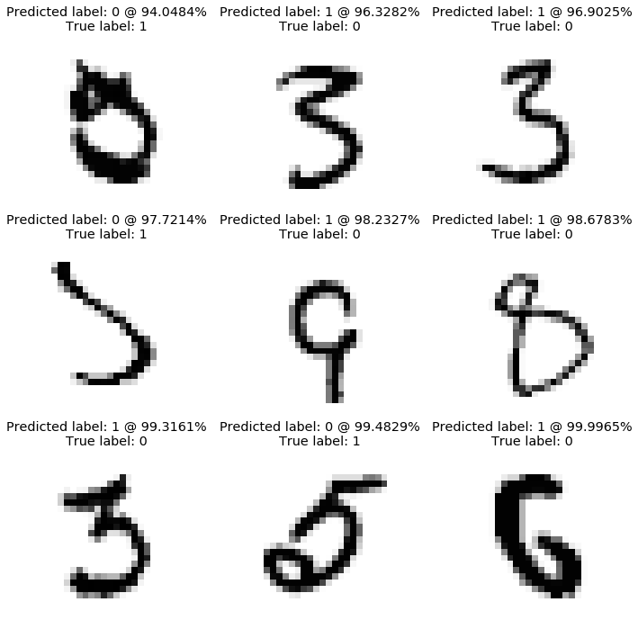
The final accuracy obtained on the test set is 98.37%. Let’s plot the worst predictions. This can help identify recurring mistakes made by the model.
# display incorrect predictions
def plot_worst_predictions(model,X_set,y_true):
    """
    Plot predictions with largest errors.

    Input:
        model: sklearn model or keras model (needs to contain a .predict function)
        X_set as np.array, shape N x M x M
        y_true as np.array, shape N x 10

    Output:
        3x3 plots of images leading to the worst predictions.
    """

    # predict the values from the validation dataset
    # size: N x 10
    y_pred = model.predict(X_set)

    # convert predictions classes to one hot vectors
    # size: N x 1
    y_pred_classes = y_pred > 0.5

    # extract errors
    # size: K x 1
    errors = (y_pred_classes - y_true != 0)

    # filter predicted classes with errors
    # size: K x 1
    y_pred_classes_errors = y_pred_classes[errors]

    # filter predictions with errors
    # size: K x 10
    y_pred_errors = y_pred[errors]

    # filter true label with errors
    # size: K x 1
    y_true_errors = y_true[errors]

    # filter records leading to errors
    # size: K x M x M
    X_set_errors = X_set[errors[:,0]]

    # probabilities of the wrong predicted numbers
    # size: K x 1
    y_pred_errors_prob = np.abs(y_true_errors - y_pred_errors)

    # difference between the probability of the predicted label and the true label
    # size: K x 1
    delta_pred_true_errors = y_pred_errors_prob

    # sorted list of the delta prob errors
    # size: K x 1
    sorted_detla_errors = np.argsort(delta_pred_true_errors)

    # Top 9 errors
    # size: 9 x 1
    most_important_errors = sorted_detla_errors[-9:]

    # plot parameters
    n = 0
    nrows = 3
    ncols = 3

    # figure
    fig, ax = plt.subplots(nrows,ncols,sharex=True,sharey=True,figsize=(12,12))

    # plot worst predictions
    for row in range(nrows):
        for col in range(ncols):

            # isolate example
            error = most_important_errors[n]

            # plot image
            ax[row,col].imshow((X_set_errors[error]).reshape((28,28)),cmap='Greys', vmin=0, vmax=1)

            # set title
            ax[row,col].set_title("Predicted label: {} @ {:.4f}%\nTrue label: {}".format(int(y_pred_classes_errors[error]),
                                                                                    y_pred_errors_prob[error]*100,
                                                                                    int(y_true_errors[error])))
            n += 1

            ax[row,col].axis('off')
plot_worst_predictions(model,X_test.T, Y_test.T)
6. Softmax Regression
In the first half of this presentation, we only cover the structure of a Deep Neural Network for binary classification. In this last portion, we will adjust our code to be able to train a multi-class classifier (i.e. softmax classifier). To do so, the following notions need to be introduced:
- One-hot encoding
- Softmax
- New cost function
Previously, the prediction for the \(i^{th}\) example \(\bar{y_{(i)}}\) was a float comprise between 0 and 1. In the softmax regression, the estimated quantity is now a vector of length \(n_{c}\) where \(n_{c}\) is the number of possible classes. Therefore, it is necessary to encode the input vector y based on the assigned class. For instance, if \(n_{c}=4\), with classes being defined as (0, 1, 2, 3) and \(y_{(i)}=2\) then the encoded vector is: \(\begin{pmatrix} 0 & 0 & 1 & 0 \end{pmatrix}\)
In addition, the activation function of the output layer needs to be modified. Instead of using the sigmoid function, we now use the softmax function defined as: \(g(x_{i}) = \frac{e^{x_{i}}}{\sum_{k=1}^{N} e^{x_{k}}}\)
Finally, the Loss Function function needs to be revised:
\[L(a^{(i)}, y^{(i)})=-y^{(i)}\log\left(a^{(i)}\right)\]Finally, the backward propagation needs to be adjusted as follows: \(dZ^{[l]} = \hat{Y} - Y\)
def softmax(Z):
    """
    Implements the softmax activation in numpy

    Arguments:
    Z -- numpy array of any shape (x, y)

    Returns:
    A -- output of softmax(z), shape (1, y)
    cache -- returns Z as well, useful during back-propagation
    """
    cache = Z
    Z -= np.max(Z)

    A = (np.exp(Z) / np.sum(np.exp(Z), axis=0))
    cache = Z

    return A, cache
def linear_activation_forward(A_prev, W, b, activation):
    """
    Implement the forward propagation for the LINEAR->ACTIVATION layer

    Arguments:
    A_prev -- activations from previous layer (or input data): (size of previous layer, number of examples)
    W -- weights matrix: numpy array of shape (size of current layer, size of previous layer)
    b -- bias vector, numpy array of shape (size of the current layer, 1)
    activation -- the activation to be used in this layer, stored as a text string: "sigmoid" or "relu" or "softmax"

    Returns:
    A -- the output of the activation function, also called the post-activation value
    cache -- a python dictionary containing "linear_cache" and "activation_cache";
             stored for computing the backward pass efficiently
    """

    if activation == "sigmoid":
        # Inputs: "A_prev, W, b". Outputs: "A, activation_cache".
        Z, linear_cache = linear_forward(A_prev, W, b)
        A, activation_cache = sigmoid(Z)

    elif activation == "relu":
        # Inputs: "A_prev, W, b". Outputs: "A, activation_cache".
        Z, linear_cache = linear_forward(A_prev, W, b)
        A, activation_cache = relu(Z)

    elif activation == "softmax":
        # Inputs: "A_prev, W, b". Outputs: "A, activation_cache".
        Z, linear_cache = linear_forward(A_prev, W, b)
        A, activation_cache = softmax(Z)

    assert (A.shape == (W.shape[0], A_prev.shape[1]))
    cache = (linear_cache, activation_cache)

    return A, cache
def L_model_forward(X, parameters):
    """
    Implement forward propagation for the [LINEAR->RELU]*(L-1)->LINEAR->SOFTMAX computation

    Arguments:
    X -- data, numpy array of shape (input size, number of examples)
    parameters -- output of initialize_parameters_deep()

    Returns:
    AL -- last post-activation value
    caches -- list of caches containing:
                every cache of linear_activation_forward() (there are L-1 of them, indexed from 0 to L-1)
    """

    caches = []
    A = X
    L = len(parameters) // 2                  # number of layers in the neural network

    # Implement [LINEAR -> RELU]*(L-1). Add "cache" to the "caches" list.
    for l in range(1, L):
        A_prev = A

        # retrieve parameters
        W = parameters['W' + str(l)]
        b = parameters['b' + str(l)]
        activation = 'relu'

        A, cache = linear_activation_forward(A_prev, W, b, activation)
        caches.append(cache)

    # Implement LINEAR -> SIGMOID. Add "cache" to the "caches" list.

    # retrieve parameters
    W = parameters['W' + str(L)]
    b = parameters['b' + str(L)]
    activation = 'softmax'

    AL, cache = linear_activation_forward(A, W, b, activation)
    caches.append(cache)

    assert(AL.shape == (10,X.shape[1]))

    return AL, caches
def compute_cost(AL, Y):
    """
    Implement the cost function.

    Arguments:
    AL -- probability vector corresponding to your label predictions, shape (1, number of examples)
    Y -- true "label" matrix using one-hot encoding (n_c, m)

    Returns:
    cost -- cross-entropy cost
    """

    m = Y.shape[1]

    # Compute loss from aL and y.
    cost = (-1/m) * np.sum( Y * np.log(AL) )

    cost = np.squeeze(cost)      # To make sure your cost's shape is what we expect (e.g. this turns [[17]] into 17).
    assert(cost.shape == ())

    return cost
def softmax_backward(dA, cache):
    """
    Implement the backward propagation for a single SOFTMAX unit.

    Arguments:
    dA -- post-activation gradient, of any shape
    cache -- 'Z' where we store for computing backward propagation efficiently

    Returns:
    dZ -- Gradient of the cost with respect to Z
    """

    Z = cache
    Z -= np.max(Z)
    s = (np.exp(Z) / np.sum(np.exp(Z), axis=0))

    dZ = dA * s * (1 - s)

    assert (dZ.shape == Z.shape)

    return dZ
def linear_activation_backward(dA, cache, activation):
    """
    Implement the backward propagation for the LINEAR->ACTIVATION layer.

    Arguments:
    dA -- post-activation gradient for current layer l
    cache -- tuple of values (linear_cache, activation_cache) we store for computing backward propagation efficiently
    activation -- the activation to be used in this layer, stored as a text string: "sigmoid" or "relu" or "softmax"

    Returns:
    dA_prev -- Gradient of the cost with respect to the activation (of the previous layer l-1), same shape as A_prev
    dW -- Gradient of the cost with respect to W (current layer l), same shape as W
    db -- Gradient of the cost with respect to b (current layer l), same shape as b
    """
    # retrieve caches
    # linear_cache = (A, W, b)
    # activation_cache = Z

    linear_cache, activation_cache = cache

    if activation == "relu":

        # parameters
        Z = activation_cache

        dZ = relu_backward(dA, Z)
        dA_prev, dW, db = linear_backward(dZ, linear_cache)

    elif activation == "sigmoid":

        # parameters
        Z = activation_cache

        dZ = sigmoid_backward(dA, Z)
        dA_prev, dW, db = linear_backward(dZ, linear_cache)

    elif activation == "softmax":

        # parameters
        Z = activation_cache

        dZ = softmax_backward(dA, Z)
        dA_prev, dW, db = linear_backward(dZ, linear_cache)

    return dA_prev, dW, db
def L_model_backward(AL, Y, caches):
    """
    Implement the backward propagation for the [LINEAR->RELU] * (L-1) -> LINEAR -> SOFTMAX group

    Arguments:
    AL -- probability vector, output of the forward propagation (L_model_forward())
    Y -- true "label" vector with one-hot encoding
    caches -- list of caches containing:
                every cache of linear_activation_forward() with "relu" (it's caches[l], for l in range(L-1) i.e l = 0...L-2)
                the cache of linear_activation_forward() with "sigmoid" (it's caches[L-1])

                for every cache, a tuple is used to store: (linear_cache, activation_cache)
                    linear_cache = (A, W, b)
                    activation_cache = Z

    Returns:
    grads -- A dictionary with the gradients
             grads["dA" + str(l)] = ...
             grads["dW" + str(l)] = ...
             grads["db" + str(l)] = ...
    """
    grads = {}
    L = len(caches) # the number of layers
    m = AL.shape[1]
    Y = Y.reshape(AL.shape) # after this line, Y is the same shape as AL

    # Initializing the back propagation
    dAL = - (np.divide(Y, AL) - np.divide(1 - Y, 1 - AL))

    # Lth layer (SIGMOID -> LINEAR) gradients. Inputs: "dAL, current_cache". Outputs: "grads["dAL-1"], grads["dWL"], grads["dbL"]
    current_cache = caches[-1]
    grads["dA" + str(L-1)], grads["dW" + str(L)], grads["db" + str(L)] = linear_activation_backward(dAL, current_cache, 'softmax')

    # Loop from l=L-2 to l=0
    for l in reversed(range(L-1)):
        # lth layer: (RELU -> LINEAR) gradients.
        # Inputs: "grads["dA" + str(l + 1)], current_cache". Outputs: "grads["dA" + str(l)] , grads["dW" + str(l + 1)] , grads["db" + str(l + 1)]
        current_cache = caches[l]
        dA_prev_temp, dW_temp, db_temp = linear_activation_backward(grads["dA" + str(l+1)], current_cache, 'relu')
        grads["dA" + str(l)] = dA_prev_temp
        grads["dW" + str(l + 1)] = dW_temp
        grads["db" + str(l + 1)] = db_temp

    return grads
def L_layer_model_multi_class(X, Y, layers_dims, learning_rate = 0.075, num_iterations = 3000, print_cost=False):
    """
    Implements a L-layer neural network: [LINEAR->RELU]*(L-1)->LINEAR->SIGMOID.

    Arguments:
    X -- data, numpy array of shape (number of examples, num_px * num_px * 3)
    Y -- true "label" vector (containing 0 or 1 if), of shape (1, number of examples)
    layers_dims -- list containing the input size and each layer size, of length (number of layers + 1).
    learning_rate -- learning rate of the gradient descent update rule
    num_iterations -- number of iterations of the optimization loop
    print_cost -- if True, it prints the cost every 100 steps

    Returns:
    parameters -- parameters learned by the model. They can then be used to predict.
    """

    np.random.seed(1)
    costs = []                         # keep track of cost

    # Parameters initialization. (≈ 1 line of code)
    parameters = initialize_parameters_deep(layers_dims)

    # Loop (gradient descent)
    for i in range(0, num_iterations):

        # Forward propagation: [LINEAR -> RELU]*(L-1) -> LINEAR -> SOFTMAX.
        AL, caches = L_model_forward(X, parameters)

        # Compute cost.
        cost = compute_cost(AL, Y)

        # Backward propagation.
        grads = L_model_backward(AL, Y, caches)

        # Update parameters.
        parameters = update_parameters(parameters, grads, learning_rate)

        # Print the cost every 100 training example
        if print_cost and i % 100 == 0:
            print ("Cost after iteration %i: %f" %(i, cost))
        if print_cost and i % 100 == 0:
            costs.append(cost)

    # plot the cost
    if print_cost:
        print(np.squeeze(costs))
        plt.plot(np.squeeze(costs))
        plt.ylabel('cost')
        plt.xlabel('iterations (per tens)')
        plt.title("Learning rate =" + str(learning_rate))
        plt.show()

    return parameters
def predict_multi(X, y_hot, y_true, parameters):
    """
    This function is used to predict the results of a  L-layer neural network.

    Arguments:
    X -- data set of examples you would like to label
    parameters -- parameters of the trained model

    Returns:
    p -- predictions for the given dataset X
    """

    m = X.shape[1]
    n = len(parameters) // 2 # number of layers in the neural network

    # Forward propagation
    probas, caches = L_model_forward(X, parameters)

    # convert probas to 0/1 predictions
    predictions = np.argmax(probas,axis=0)

    # print results
    print("\tAccuracy: {:.2f}%%".format(np.sum((predictions == y_true))/m*100))

    return predictions
7. Application of Multi-class on MNIST
Now that our model is capable of handling multi-class model, let’s test it against the MNIST dataset but this time, we keep all the classes instead of only predicting “5” or “not 5”.
def onehot(Y, n_class):
    '''
    Return one-hot encoding of the Y array
    '''
    Y_hot = np.eye(n_class)[Y.reshape(-1)]

    return Y_hot
# load data and create train and test sets
mnist = tf.keras.datasets.mnist
(X_train, Y_train), (X_test, Y_test) = mnist.load_data()

# reshape
X_train = X_train.reshape(-1,28*28).T
X_test = X_test.reshape(-1,28*28).T

Y_train = Y_train.reshape(1,-1)
Y_test = Y_test.reshape(1,-1)

# normalize
X_train = X_train / 255.0
X_test = X_test / 255.0

# count unique class
n_class = len(np.unique(Y_train))

# one-hot-encoding
Y_train_hot = onehot(Y_train, n_class).T
Y_test_hot = onehot(Y_test, n_class).T
When creating our model geometry, the output layer now has to be defined with 10 output units. Each unit corresponds to one possible output class (0 to 9).
# three candidates are defined
models = {
    '28x28->10':[28*28, 10],
    '28x28->28->10':[28*28, 28, 10],
    '28x28->28->10->10':[28*28, 28, 10, 10],
}
scores = {}

# test all three models against the train and test sets
for name, layers_dims in models.items():

    # generate model
    parameters = L_layer_model_multi_class(X_train,
                                           Y_train_hot,
                                           layers_dims,
                                           num_iterations = 3000,
                                           print_cost = False)

    # print name
    print('\n'+name)

    # make predictions on train set
    print('Accuracy on train set:\t')
    pred_train = predict_multi(X_train, Y_train_hot, Y_train, parameters)

    # make predictions on test set
    print('Accuracy on test set:\t')
    pred_test = predict_multi(X_test, Y_test_hot, Y_test, parameters)
28x28->10
Accuracy on train set:
	Accuracy: 91.42%%
Accuracy on test set:
	Accuracy: 91.72%%

28x28->28->10
Accuracy on train set:
	Accuracy: 93.96%%
Accuracy on test set:
	Accuracy: 93.89%%

28x28->28->10->10
Accuracy on train set:
	Accuracy: 91.71%%
Accuracy on test set:
	Accuracy: 91.47%%
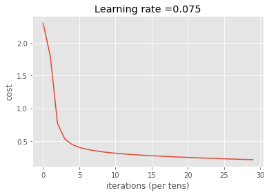
The second network (28->10) gives the best results with an accuracy on training equal to 93.96% and an accuracy on the test set equal to 93.89%. Let’s plot the worst predictions and the confusion matrix to assess the detailed performances of our model
from sklearn.metrics import confusion_matrix

best_model = L_layer_model_multi_class(X_train,
                                       Y_train_hot,
                                       [28*28, 28, 10],
                                       num_iterations = 3000,
                                       print_cost = True)
Cost after iteration 0: 2.302698
Cost after iteration 100: 1.797392
Cost after iteration 200: 0.767258
Cost after iteration 300: 0.532965
Cost after iteration 400: 0.447355
Cost after iteration 500: 0.403150
Cost after iteration 600: 0.374832
Cost after iteration 700: 0.354289
Cost after iteration 800: 0.338238
Cost after iteration 900: 0.325133
Cost after iteration 1000: 0.314092
Cost after iteration 1100: 0.304642
Cost after iteration 1200: 0.296369
Cost after iteration 1300: 0.288986
Cost after iteration 1400: 0.282327
Cost after iteration 1500: 0.276215
Cost after iteration 1600: 0.270472
Cost after iteration 1700: 0.265039
Cost after iteration 1800: 0.259864
Cost after iteration 1900: 0.254887
Cost after iteration 2000: 0.250102
Cost after iteration 2100: 0.245551
Cost after iteration 2200: 0.241226
Cost after iteration 2300: 0.237107
Cost after iteration 2400: 0.233160
Cost after iteration 2500: 0.229358
Cost after iteration 2600: 0.225705
Cost after iteration 2700: 0.222219
Cost after iteration 2800: 0.218869
Cost after iteration 2900: 0.215616
[2.30269797 1.7973915  0.76725844 0.53296483 0.44735486 0.40315035
 0.37483193 0.35428899 0.33823834 0.32513306 0.31409214 0.30464182
 0.29636928 0.28898567 0.28232707 0.27621464 0.27047229 0.26503943
 0.25986411 0.25488744 0.25010213 0.24555082 0.24122609 0.23710707
 0.23316011 0.22935838 0.22570514 0.22221895 0.21886946 0.21561591]
def plot_worst_predictions(X_set,y_true, y_pred, grid = 3):
    """
    Plot predictions with largest errors.

    Input:
        model: sklearn model or keras model (needs to contain a .predict function)
        X_set as np.array, shape N x M x M
        y_true as np.array, shape 10 x N

    Output:
        3x3 plots of images leading to the worst predictions.
    """

    # convert predictions classes to one hot vectors
    # size: 1 x N
    y_pred_classes = np.argmax(y_pred,axis = 0).reshape((1,-1))
    assert y_true.shape == y_pred.shape
    #print('y_pred_classes',y_pred_classes.shape)
    #print('y_pred',y_pred.shape)

    # convert y_true one-hot to classes
    y_true_classes = np.argmax(y_true, axis = 0).reshape((1,-1))
    assert y_true_classes.shape == y_pred_classes.shape
    #print('y_true_classes',y_true_classes.shape)

    # extract errors
    # size: 1 x K
    errors = (y_pred_classes - y_true_classes != 0)
    #print('errors',errors.shape)

    # filter predicted classes with errors
    # size: 1 x K
    y_pred_classes_errors = y_pred_classes[0,errors[0,:]].reshape((1,-1))
    #print('y_pred_classes_errors',y_pred_classes_errors.shape)

    # filter predictions with errors
    # size: 10 x K
    y_pred_errors = y_pred[:,errors[0,:]]
    #print('y_pred_errors',y_pred_errors.shape)

    # filter true label with errors
    # size: 10 x K
    y_true_errors = y_true_classes[:,errors[0,:]]
    #print('y_true_errors',y_true_errors.shape)

    # filter records leading to errors
    # size: M x M x K
    X_set_errors = X_set.reshape((28, 28, -1))
    X_set_errors = X_set_errors[:,:,errors[0,:]]
    #print('X_set_errors',X_set_errors.shape)

    # probabilities of the wrong predicted numbers
    # size: 1 x K
    y_pred_errors_prob = np.max(y_pred_errors,axis = 0).reshape((1,-1))
    #print('y_pred_errors_prob',y_pred_errors_prob.shape)

    # predicted probabilities of the true values in the error set
    # np.take: Take elements from an array along an axis.
    # >>> a = [4, 3, 5, 7, 6, 8]
    # >>> indices = [0, 1, 4]
    # >>> np.take(a, indices)
    # array([4, 3, 6])
    # np.take re-organize the columns
    # use np.diagonal to only extract the desired predictions
    # size: 1 x K
    true_prob_errors = np.diagonal(np.take(y_pred_errors, y_true_errors, axis=0)).T
    #print('true_prob_errors',true_prob_errors.shape)

    # difference between the probability of the predicted label and the true label
    # size: K x 1
    delta_pred_true_errors = y_pred_errors_prob - true_prob_errors
    #print('delta_pred_true_errors',delta_pred_true_errors.shape)

    # sorted list of the delta prob errors
    # size: 1 x K
    sorted_detla_errors = np.argsort(delta_pred_true_errors)
    #print('sorted_detla_errors',sorted_detla_errors.shape)

    # Top 9 errors
    # size: 9 x 1
    most_important_errors = sorted_detla_errors[0,-grid*grid:]

    # plot parameters
    n = 0
    nrows = grid
    ncols = grid

    # figure
    fig, ax = plt.subplots(nrows,ncols,sharex=True,sharey=True,figsize=(grid*4,grid*4))

    # plot worst predictions
    for row in range(nrows):
        for col in range(ncols):

            # isolate example
            error = most_important_errors[n]

            # plot image
            ax[row,col].imshow((X_set_errors[:,:,error]).reshape((28,28)),cmap='Greys', vmin=0, vmax=1)

            # set title
            ax[row,col].set_title("Predicted label: {} @ {:.0f}%\nTrue label: {}".format(y_pred_classes_errors[0,error],
                                                                                    y_pred_errors_prob[0,error]*100,
                                                                                    y_true_errors[0,error]))
            n += 1

            ax[row,col].axis('off')
# Make Predictions on test set and train set
probas_test, caches = L_model_forward(X_test, parameters)

probas_train, caches = L_model_forward(X_train, parameters)
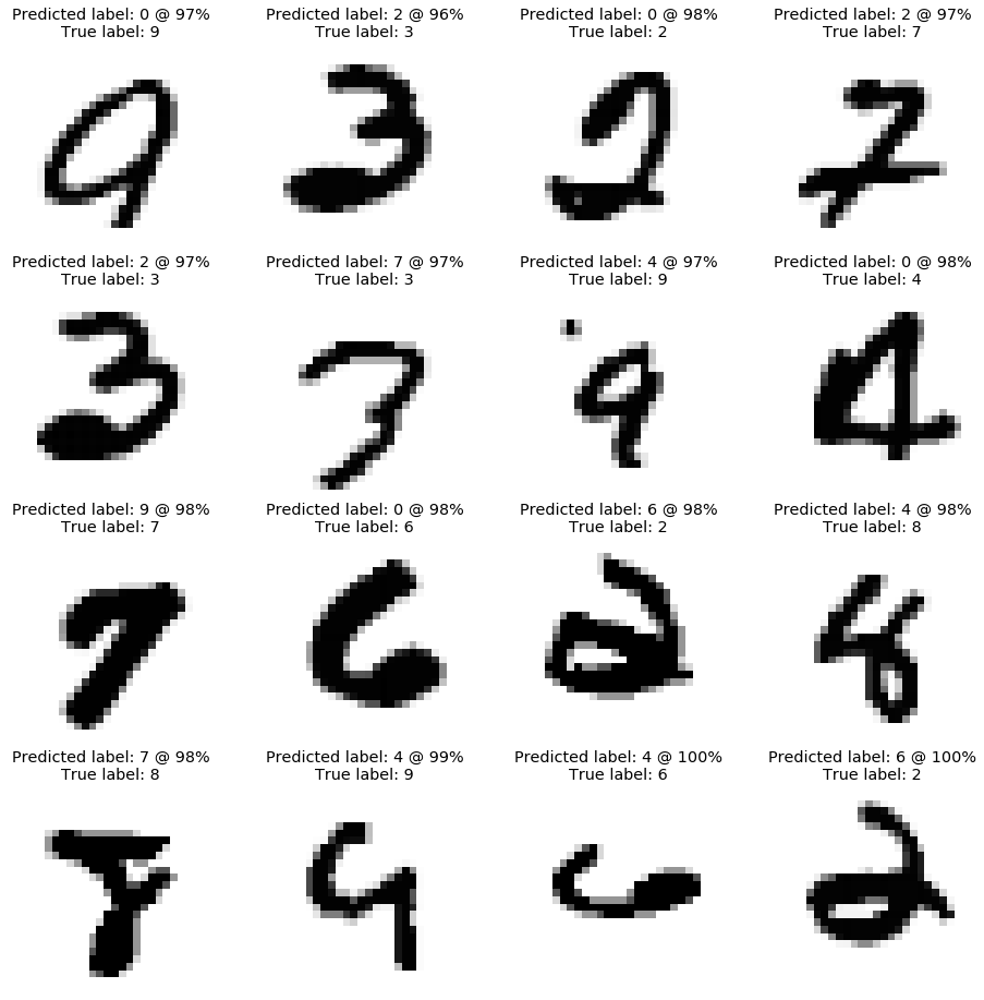
As shown below, the model makes mistakes on relatively complicated examples. Some of the digits shown below can be easily mistaken even when categorized by humans.
# Display the worst predictions
plot_worst_predictions(X_test, Y_test_hot, probas_test, grid=4)
# Plot confusion matrix
from sklearn.metrics import confusion_matrix
from sklearn.utils.multiclass import unique_labels

def plot_confusion_matrix(y_true, y_pred, classes, normalize=False, title=None, cmap=plt.cm.Blues):
    """
    This function prints and plots the confusion matrix.
    Normalization can be applied by setting `normalize=True`.
    """
    np.set_printoptions(precision=2)

    if not title:
        if normalize:
            title = 'Normalized confusion matrix'
        else:
            title = 'Confusion matrix, without normalization'

    # Compute confusion matrix
    cm = confusion_matrix(y_true, y_pred)

    # Only use the labels that appear in the data
    classes = classes[unique_labels(y_true, y_pred)]
    if normalize:
        cm = cm.astype('float') / cm.sum(axis=1)[:, np.newaxis]

    fig, ax = plt.subplots(figsize=(10,10))
    ax.grid(False)
    im = ax.imshow(cm, interpolation='nearest', cmap=cmap)
    ax.figure.colorbar(im, ax=ax, shrink=0.5)

    # We want to show all ticks...
    ax.set(xticks=np.arange(cm.shape[1]),
           yticks=np.arange(cm.shape[0]),
           # ... and label them with the respective list entries
           xticklabels=classes, yticklabels=classes,
           title=title,
           ylabel='True label',
           xlabel='Predicted label')

    # Rotate the tick labels and set their alignment.
    plt.setp(ax.get_xticklabels(), rotation=45, ha="right",
             rotation_mode="anchor")

    # Loop over data dimensions and create text annotations.
    fmt = '.2f' if normalize else 'd'
    thresh = cm.max() / 2.
    for i in range(cm.shape[0]):
        for j in range(cm.shape[1]):
            ax.text(j, i, format(cm[i, j], fmt),
                    ha="center", va="center",
                    color="white" if cm[i, j] > thresh else "black")
    fig.tight_layout()
    return ax
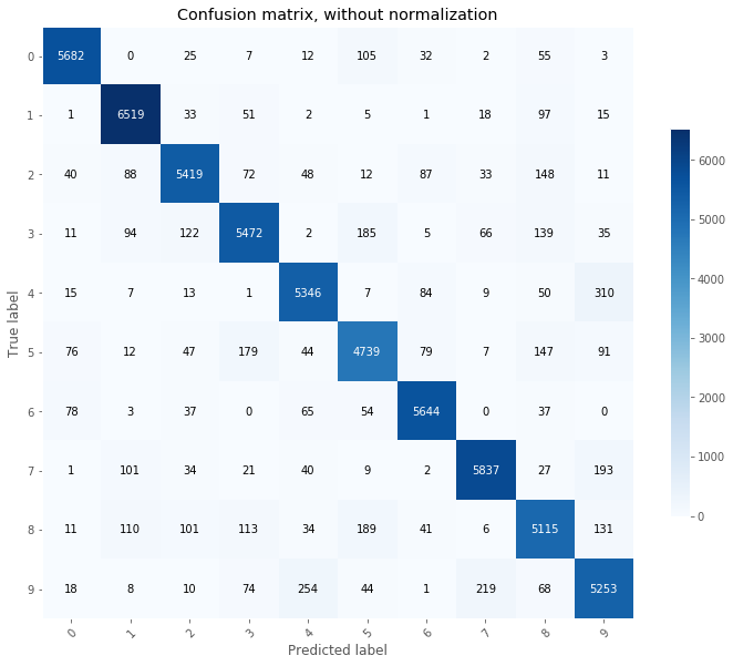
When working on classifier, confusion matrices are a great tool to identify potential for improvements. Predictions are made on the train and test set and confusion matrices are plotted.
# Confusion matrix on training set
plot_confusion_matrix(Y_train.T, np.argmax(probas_train, axis=0).T, classes = np.array(range(10)));
# Confusion matrix on training set
plot_confusion_matrix(Y_test.T, np.argmax(probas_test, axis=0).T, classes = np.array(range(10)));
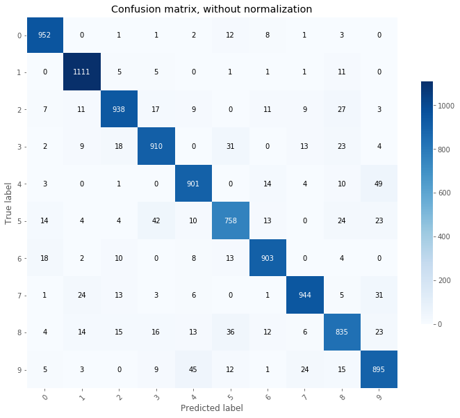
From the above, we can see that the most common mistakes made on the test set are:
- 4 predicted as 9
- 9 predicted as 4
- 5 predicted as 3
From the above, we can decide to add more focusing on reducing the errors made on the 4, 9, and 5 classes by adding more training images for these classes.
8. Conclusion
The deep neural network proved to be an improvement on the single layer model. There are a few aspects to keep in mind when using this architecture:
- Complex models are prone to over-fitting. Indeed, with more parameters, a complex model can over-fit the training data.
- Complex models require more processing power.
- The architecture of the DNN needs can take many shapes. From deep model (large number of layers) to wide models (large number of hidden units), the architecture of a network needs to be tested and tuned.
Final words on regularization and optimization:
In order to reduce the over-fitting, there exists a set of techniques called regularization. Their role in to prevent the model from over-learning the training data by simplifying the model. The most common ones are:
L1 and L2 regularizations
The cost function is modified and a penalty term is added:
The idea behind this strategy is to ensure that the model is not governed by a small subsets of weights with high values. The parameter lambda is tunable.
Dropout
Similar to L1 and L2 regularizations, Dropout prevents the model to rely on a subset of weights. During training, a small portion of the hidden units in each layer are randomly set to 0. The rest of the weights are scaled to account for the dropout. By randomly removing hidden units from the model, dropout forces the model to distribute its learning power across multiple paths instead of a few preferred ones.
Early stopping
The model is trained and after each epoch, a metric (accuracy) is computed on a validation set. The training is stopped when a condition on the metric is reached. This can be defined as “accuracy decreases” or “accuracy reaches a certain threshold”.
Data augmentation
Data augmentation consists of artificially generate more training data by using the original training dataset. When working with images, transformation such as zooming, shifting, color-change, rotation are applied randomly to generate more images. This will help the model to train on more cases and better perform when making predictions using unseen data.