Forest Cover Type
We are asked to predict the forest cover type (the predominant kind of tree cover) from cartographic variables. The actual forest cover type for a given 30 x 30 meter cell was determined from US Forest Service (USFS) Region 2 Resource Information System data. Independent variables were then derived from data obtained from the US Geological Survey and USFS. The data is in raw form and contains binary columns of data for qualitative independent variables such as wilderness areas and soil type.
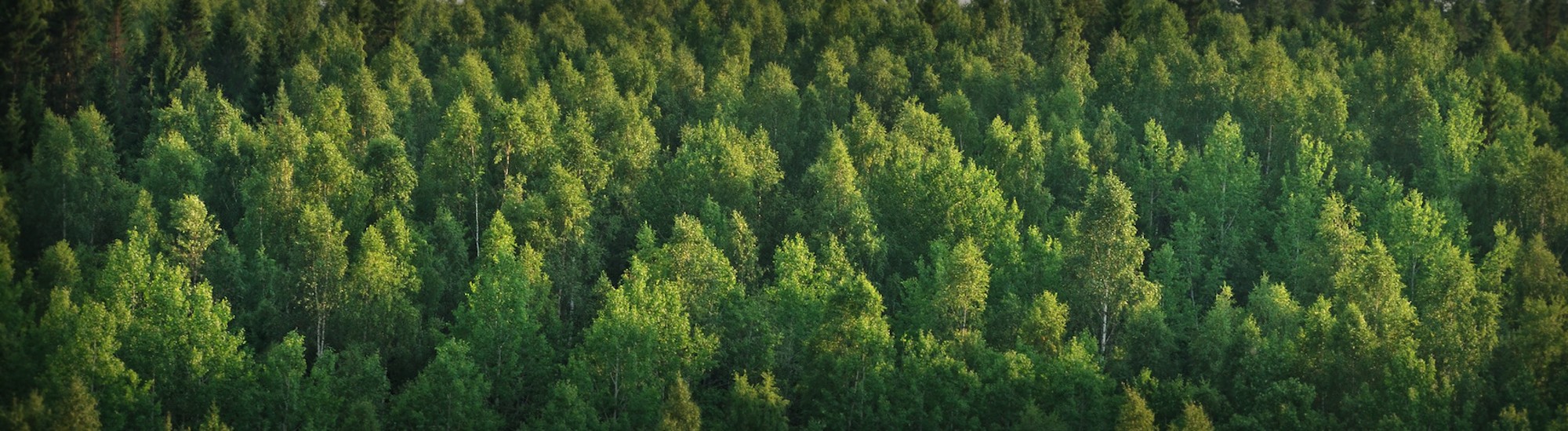
This study area includes four wilderness areas located in the Roosevelt National Forest of northern Colorado. These areas represent forests with minimal human-caused disturbances, so that existing forest cover types are more a result of ecological processes rather than forest management practices.
The pictures below show the seven cover types considered in this analysis
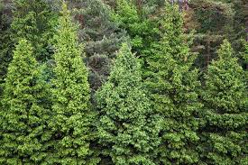
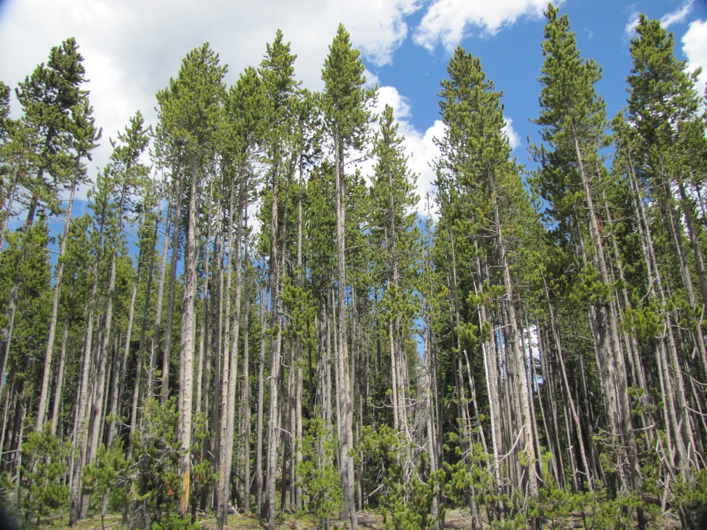
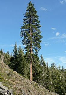
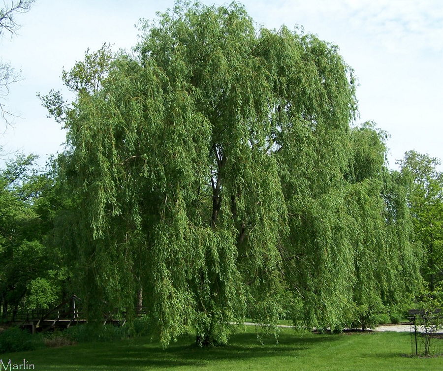
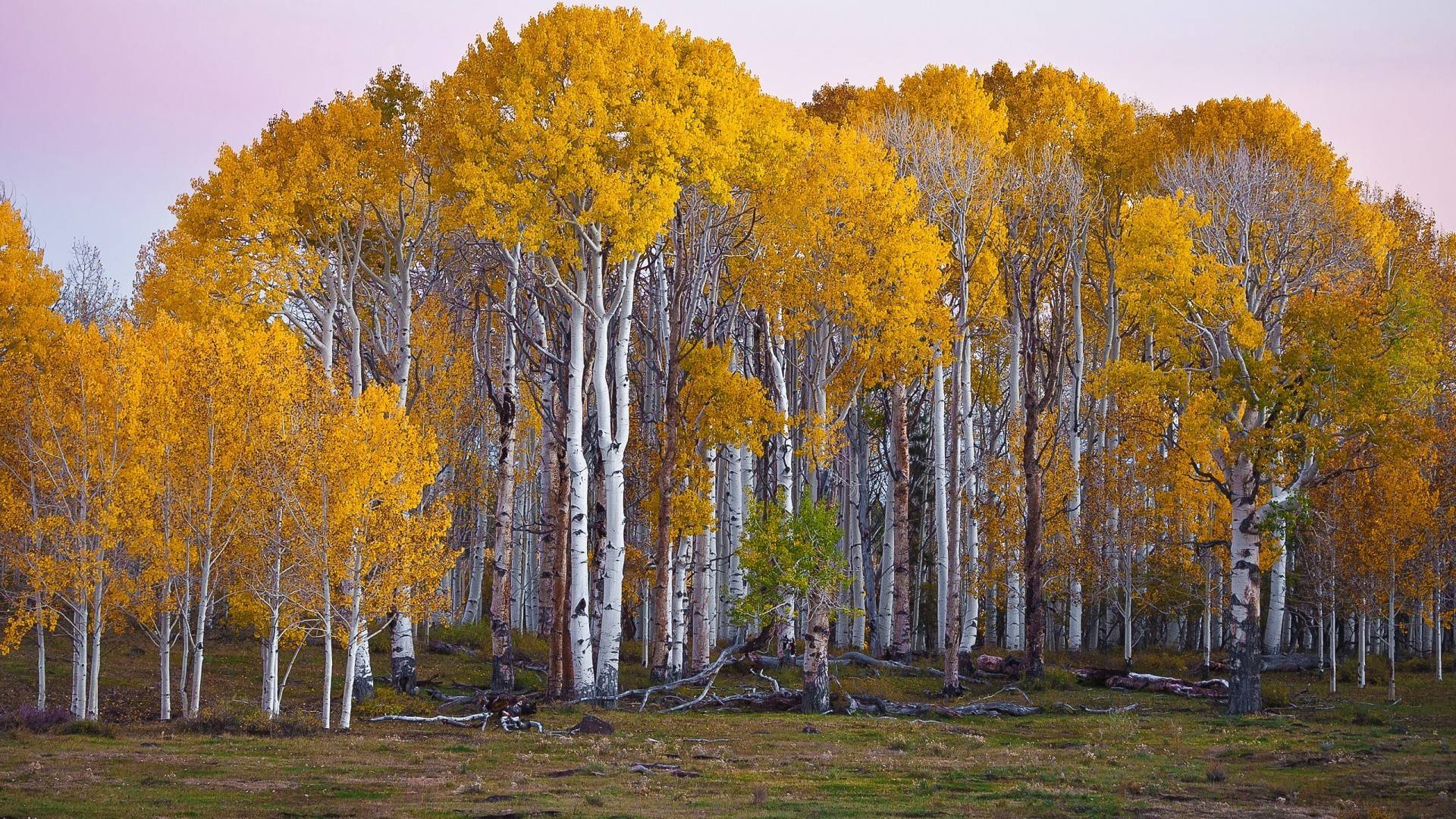
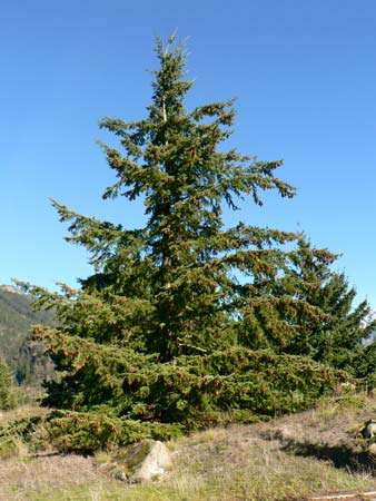
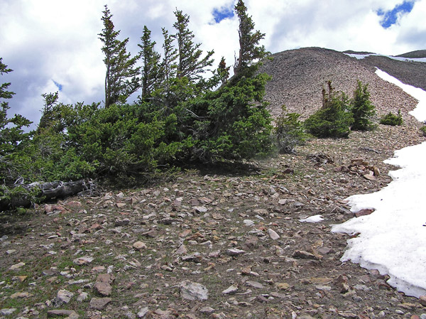
Table of Content
1. Introduction
2. Tool Functions
3. Data Exploration
3.1 Class Distribution
3.2 Elevation
3.3 Aspect
3.4 Slope
3.5 Horizontal Distance To Hydrology
3.6 Vertical Distance To Hydrology
3.7 Horizontal Distance To Roadways
3.8 Hillshade 9 AM
3.9 Hillshade Noon
3.10 Hillshade 3 PM
3.11 Horizontal Distance To Fire Points
3.12 Wilderness Areas
3.13 Soil Type
3.14 Feature Correlation
4. Feature Engineering
5. Models
6. Submission
1. Introduction
# import libraries
import pandas as pd
import numpy as np
import sys
np.set_printoptions(threshold=sys.maxsize)

import matplotlib.pyplot as plt
import seaborn as sns
# sns.set_style("whitegrid")
sns.set()
mycols = ["#66c2ff", "#00cc99", "#85e085", "#ffd966", "#ffb3b3", "#dab3ff", "#c2c2d6"]
sns.set_palette(palette = mycols, n_colors = 7)

from scipy import stats
from scipy.stats import skew, norm
from scipy.special import boxcox1p
from scipy.stats.stats import pearsonr
from scipy.stats import ttest_ind

from sklearn.model_selection import GridSearchCV, ShuffleSplit

import xgboost as xgb

import math

import warnings
warnings.simplefilter(action='ignore', category=FutureWarning)
warnings.simplefilter(action='ignore', category=RuntimeWarning)
warnings.filterwarnings("ignore", category=DeprecationWarning)

from sklearn.base import TransformerMixin, BaseEstimator

decimals = 2
%matplotlib inline
The study area includes four wilderness areas located in the Roosevelt National Forest of northern Colorado. Each observation is a 30m x 30m patch. Our are asked to predict an integer classification for the forest cover type. The seven types are:
- Spruce/Fir
- Lodgepole Pine
- Ponderosa Pine
- Cottonwood/Willow
- Aspen
- Douglas-fir
- Krummholz
The training set (15120 observations) contains both features and the Cover_Type. The test set contains only the features. You must predict the Cover_Type for every row in the test set (565892 observations).
Data Fields
- Elevation - Elevation in meters
- Aspect - Aspect in degrees azimuth
- Slope - Slope in degrees
- Horizontal_Distance_To_Hydrology - Horz Dist to nearest surface water features
- Vertical_Distance_To_Hydrology - Vert Dist to nearest surface water features
- Horizontal_Distance_To_Roadways - Horz Dist to nearest roadway
- Hillshade_9am (0 to 255 index) - Hillshade index at 9am, summer solstice
- Hillshade_Noon (0 to 255 index) - Hillshade index at noon, summer solstice
- Hillshade_3pm (0 to 255 index) - Hillshade index at 3pm, summer solstice
- Horizontal_Distance_To_Fire_Points - Horz Dist to nearest wildfire ignition points
- Wilderness_Area (4 binary columns, 0 = absence or 1 = presence) - Wilderness area designation
- Soil_Type (40 binary columns, 0 = absence or 1 = presence) - Soil Type designation
- Cover_Type (7 types, integers 1 to 7) - Forest Cover Type designation
The wilderness areas are:
- Rawah Wilderness Area
- Neota Wilderness Area
- Comanche Peak Wilderness Area
- Cache la Poudre Wilderness Area
The soil types are:
- Cathedral family - Rock outcrop complex, extremely stony.
- Vanet - Ratake families complex, very stony.
- Haploborolis - Rock outcrop complex, rubbly.
- Ratake family - Rock outcrop complex, rubbly.
- Vanet family - Rock outcrop complex complex, rubbly.
- Vanet - Wetmore families - Rock outcrop complex, stony.
- Gothic family.
- Supervisor - Limber families complex.
- Troutville family, very stony.
- Bullwark - Catamount families - Rock outcrop complex, rubbly.
- Bullwark - Catamount families - Rock land complex, rubbly.
- Legault family - Rock land complex, stony.
- Catamount family - Rock land - Bullwark family complex, rubbly.
- Pachic Argiborolis - Aquolis complex.
- unspecified in the USFS Soil and ELU Survey.
- Cryaquolis - Cryoborolis complex.
- Gateview family - Cryaquolis complex.
- Rogert family, very stony.
- Typic Cryaquolis - Borohemists complex.
- Typic Cryaquepts - Typic Cryaquolls complex.
- Typic Cryaquolls - Leighcan family, till substratum complex.
- Leighcan family, till substratum, extremely bouldery.
- Leighcan family, till substratum - Typic Cryaquolls complex.
- Leighcan family, extremely stony.
- Leighcan family, warm, extremely stony.
- Granile - Catamount families complex, very stony.
- Leighcan family, warm - Rock outcrop complex, extremely stony.
- Leighcan family - Rock outcrop complex, extremely stony.
- Como - Legault families complex, extremely stony.
- Como family - Rock land - Legault family complex, extremely stony.
- Leighcan - Catamount families complex, extremely stony.
- Catamount family - Rock outcrop - Leighcan family complex, extremely stony.
- Leighcan - Catamount families - Rock outcrop complex, extremely stony.
- Cryorthents - Rock land complex, extremely stony.
- Cryumbrepts - Rock outcrop - Cryaquepts complex.
- Bross family - Rock land - Cryumbrepts complex, extremely stony.
- Rock outcrop - Cryumbrepts - Cryorthents complex, extremely stony.
- Leighcan - Moran families - Cryaquolls complex, extremely stony.
- Moran family - Cryorthents - Leighcan family complex, extremely stony.
- Moran family - Cryorthents - Rock land complex, extremely stony.
# load data
train = pd.read_csv('data/train.csv')
test = pd.read_csv('data/test.csv')

# save Id
train_ID = train['Id']
test_ID = test['Id']

# drop iD
del train['Id']
del test['Id']

# investigate shapes
print('Train shape:', train.shape)
print('Test shape:', test.shape)
Train shape: (15120, 55)
Test shape: (565892, 54)
# list features
print('List of features:')
print(train.columns)
List of features:
Index(['Elevation', 'Aspect', 'Slope', 'Horizontal_Distance_To_Hydrology',
       'Vertical_Distance_To_Hydrology', 'Horizontal_Distance_To_Roadways',
       'Hillshade_9am', 'Hillshade_Noon', 'Hillshade_3pm',
       'Horizontal_Distance_To_Fire_Points', 'Wilderness_Area1',
       'Wilderness_Area2', 'Wilderness_Area3', 'Wilderness_Area4',
       'Soil_Type1', 'Soil_Type2', 'Soil_Type3', 'Soil_Type4', 'Soil_Type5',
       'Soil_Type6', 'Soil_Type7', 'Soil_Type8', 'Soil_Type9', 'Soil_Type10',
       'Soil_Type11', 'Soil_Type12', 'Soil_Type13', 'Soil_Type14',
       'Soil_Type15', 'Soil_Type16', 'Soil_Type17', 'Soil_Type18',
       'Soil_Type19', 'Soil_Type20', 'Soil_Type21', 'Soil_Type22',
       'Soil_Type23', 'Soil_Type24', 'Soil_Type25', 'Soil_Type26',
       'Soil_Type27', 'Soil_Type28', 'Soil_Type29', 'Soil_Type30',
       'Soil_Type31', 'Soil_Type32', 'Soil_Type33', 'Soil_Type34',
       'Soil_Type35', 'Soil_Type36', 'Soil_Type37', 'Soil_Type38',
       'Soil_Type39', 'Soil_Type40', 'Cover_Type'],
      dtype='object')
# explore data
print("Here are a few observations: ")
train.head()
Here are a few observations:
| Elevation | Aspect | Slope | Horizontal_Distance_To_Hydrology | Vertical_Distance_To_Hydrology | Horizontal_Distance_To_Roadways | Hillshade_9am | Hillshade_Noon | Hillshade_3pm | Horizontal_Distance_To_Fire_Points | ... | Soil_Type32 | Soil_Type33 | Soil_Type34 | Soil_Type35 | Soil_Type36 | Soil_Type37 | Soil_Type38 | Soil_Type39 | Soil_Type40 | Cover_Type | |
|---|---|---|---|---|---|---|---|---|---|---|---|---|---|---|---|---|---|---|---|---|---|
| 0 | 2596 | 51 | 3 | 258 | 0 | 510 | 221 | 232 | 148 | 6279 | ... | 0 | 0 | 0 | 0 | 0 | 0 | 0 | 0 | 0 | 5 |
| 1 | 2590 | 56 | 2 | 212 | -6 | 390 | 220 | 235 | 151 | 6225 | ... | 0 | 0 | 0 | 0 | 0 | 0 | 0 | 0 | 0 | 5 |
| 2 | 2804 | 139 | 9 | 268 | 65 | 3180 | 234 | 238 | 135 | 6121 | ... | 0 | 0 | 0 | 0 | 0 | 0 | 0 | 0 | 0 | 2 |
| 3 | 2785 | 155 | 18 | 242 | 118 | 3090 | 238 | 238 | 122 | 6211 | ... | 0 | 0 | 0 | 0 | 0 | 0 | 0 | 0 | 0 | 2 |
| 4 | 2595 | 45 | 2 | 153 | -1 | 391 | 220 | 234 | 150 | 6172 | ... | 0 | 0 | 0 | 0 | 0 | 0 | 0 | 0 | 0 | 5 |
5 rows × 55 columns
# explore data
train.info()
<class 'pandas.core.frame.DataFrame'>
RangeIndex: 15120 entries, 0 to 15119
Data columns (total 55 columns):
Elevation                             15120 non-null int64
Aspect                                15120 non-null int64
Slope                                 15120 non-null int64
Horizontal_Distance_To_Hydrology      15120 non-null int64
Vertical_Distance_To_Hydrology        15120 non-null int64
Horizontal_Distance_To_Roadways       15120 non-null int64
Hillshade_9am                         15120 non-null int64
Hillshade_Noon                        15120 non-null int64
Hillshade_3pm                         15120 non-null int64
Horizontal_Distance_To_Fire_Points    15120 non-null int64
Wilderness_Area1                      15120 non-null int64
Wilderness_Area2                      15120 non-null int64
Wilderness_Area3                      15120 non-null int64
Wilderness_Area4                      15120 non-null int64
Soil_Type1                            15120 non-null int64
Soil_Type2                            15120 non-null int64
Soil_Type3                            15120 non-null int64
Soil_Type4                            15120 non-null int64
Soil_Type5                            15120 non-null int64
Soil_Type6                            15120 non-null int64
Soil_Type7                            15120 non-null int64
Soil_Type8                            15120 non-null int64
Soil_Type9                            15120 non-null int64
Soil_Type10                           15120 non-null int64
Soil_Type11                           15120 non-null int64
Soil_Type12                           15120 non-null int64
Soil_Type13                           15120 non-null int64
Soil_Type14                           15120 non-null int64
Soil_Type15                           15120 non-null int64
Soil_Type16                           15120 non-null int64
Soil_Type17                           15120 non-null int64
Soil_Type18                           15120 non-null int64
Soil_Type19                           15120 non-null int64
Soil_Type20                           15120 non-null int64
Soil_Type21                           15120 non-null int64
Soil_Type22                           15120 non-null int64
Soil_Type23                           15120 non-null int64
Soil_Type24                           15120 non-null int64
Soil_Type25                           15120 non-null int64
Soil_Type26                           15120 non-null int64
Soil_Type27                           15120 non-null int64
Soil_Type28                           15120 non-null int64
Soil_Type29                           15120 non-null int64
Soil_Type30                           15120 non-null int64
Soil_Type31                           15120 non-null int64
Soil_Type32                           15120 non-null int64
Soil_Type33                           15120 non-null int64
Soil_Type34                           15120 non-null int64
Soil_Type35                           15120 non-null int64
Soil_Type36                           15120 non-null int64
Soil_Type37                           15120 non-null int64
Soil_Type38                           15120 non-null int64
Soil_Type39                           15120 non-null int64
Soil_Type40                           15120 non-null int64
Cover_Type                            15120 non-null int64
dtypes: int64(55)
memory usage: 6.3 MB
# explore data
test.info()
<class 'pandas.core.frame.DataFrame'>
RangeIndex: 565892 entries, 0 to 565891
Data columns (total 54 columns):
Elevation                             565892 non-null int64
Aspect                                565892 non-null int64
Slope                                 565892 non-null int64
Horizontal_Distance_To_Hydrology      565892 non-null int64
Vertical_Distance_To_Hydrology        565892 non-null int64
Horizontal_Distance_To_Roadways       565892 non-null int64
Hillshade_9am                         565892 non-null int64
Hillshade_Noon                        565892 non-null int64
Hillshade_3pm                         565892 non-null int64
Horizontal_Distance_To_Fire_Points    565892 non-null int64
Wilderness_Area1                      565892 non-null int64
Wilderness_Area2                      565892 non-null int64
Wilderness_Area3                      565892 non-null int64
Wilderness_Area4                      565892 non-null int64
Soil_Type1                            565892 non-null int64
Soil_Type2                            565892 non-null int64
Soil_Type3                            565892 non-null int64
Soil_Type4                            565892 non-null int64
Soil_Type5                            565892 non-null int64
Soil_Type6                            565892 non-null int64
Soil_Type7                            565892 non-null int64
Soil_Type8                            565892 non-null int64
Soil_Type9                            565892 non-null int64
Soil_Type10                           565892 non-null int64
Soil_Type11                           565892 non-null int64
Soil_Type12                           565892 non-null int64
Soil_Type13                           565892 non-null int64
Soil_Type14                           565892 non-null int64
Soil_Type15                           565892 non-null int64
Soil_Type16                           565892 non-null int64
Soil_Type17                           565892 non-null int64
Soil_Type18                           565892 non-null int64
Soil_Type19                           565892 non-null int64
Soil_Type20                           565892 non-null int64
Soil_Type21                           565892 non-null int64
Soil_Type22                           565892 non-null int64
Soil_Type23                           565892 non-null int64
Soil_Type24                           565892 non-null int64
Soil_Type25                           565892 non-null int64
Soil_Type26                           565892 non-null int64
Soil_Type27                           565892 non-null int64
Soil_Type28                           565892 non-null int64
Soil_Type29                           565892 non-null int64
Soil_Type30                           565892 non-null int64
Soil_Type31                           565892 non-null int64
Soil_Type32                           565892 non-null int64
Soil_Type33                           565892 non-null int64
Soil_Type34                           565892 non-null int64
Soil_Type35                           565892 non-null int64
Soil_Type36                           565892 non-null int64
Soil_Type37                           565892 non-null int64
Soil_Type38                           565892 non-null int64
Soil_Type39                           565892 non-null int64
Soil_Type40                           565892 non-null int64
dtypes: int64(54)
memory usage: 233.1 MB
# explore data
train.describe()
| Elevation | Aspect | Slope | Horizontal_Distance_To_Hydrology | Vertical_Distance_To_Hydrology | Horizontal_Distance_To_Roadways | Hillshade_9am | Hillshade_Noon | Hillshade_3pm | Horizontal_Distance_To_Fire_Points | ... | Soil_Type32 | Soil_Type33 | Soil_Type34 | Soil_Type35 | Soil_Type36 | Soil_Type37 | Soil_Type38 | Soil_Type39 | Soil_Type40 | Cover_Type | |
|---|---|---|---|---|---|---|---|---|---|---|---|---|---|---|---|---|---|---|---|---|---|
| count | 15120.000000 | 15120.000000 | 15120.000000 | 15120.000000 | 15120.000000 | 15120.000000 | 15120.000000 | 15120.000000 | 15120.000000 | 15120.000000 | ... | 15120.000000 | 15120.000000 | 15120.000000 | 15120.000000 | 15120.000000 | 15120.000000 | 15120.000000 | 15120.000000 | 15120.000000 | 15120.000000 |
| mean | 2749.322553 | 156.676653 | 16.501587 | 227.195701 | 51.076521 | 1714.023214 | 212.704299 | 218.965608 | 135.091997 | 1511.147288 | ... | 0.045635 | 0.040741 | 0.001455 | 0.006746 | 0.000661 | 0.002249 | 0.048148 | 0.043452 | 0.030357 | 4.000000 |
| std | 417.678187 | 110.085801 | 8.453927 | 210.075296 | 61.239406 | 1325.066358 | 30.561287 | 22.801966 | 45.895189 | 1099.936493 | ... | 0.208699 | 0.197696 | 0.038118 | 0.081859 | 0.025710 | 0.047368 | 0.214086 | 0.203880 | 0.171574 | 2.000066 |
| min | 1863.000000 | 0.000000 | 0.000000 | 0.000000 | -146.000000 | 0.000000 | 0.000000 | 99.000000 | 0.000000 | 0.000000 | ... | 0.000000 | 0.000000 | 0.000000 | 0.000000 | 0.000000 | 0.000000 | 0.000000 | 0.000000 | 0.000000 | 1.000000 |
| 25% | 2376.000000 | 65.000000 | 10.000000 | 67.000000 | 5.000000 | 764.000000 | 196.000000 | 207.000000 | 106.000000 | 730.000000 | ... | 0.000000 | 0.000000 | 0.000000 | 0.000000 | 0.000000 | 0.000000 | 0.000000 | 0.000000 | 0.000000 | 2.000000 |
| 50% | 2752.000000 | 126.000000 | 15.000000 | 180.000000 | 32.000000 | 1316.000000 | 220.000000 | 223.000000 | 138.000000 | 1256.000000 | ... | 0.000000 | 0.000000 | 0.000000 | 0.000000 | 0.000000 | 0.000000 | 0.000000 | 0.000000 | 0.000000 | 4.000000 |
| 75% | 3104.000000 | 261.000000 | 22.000000 | 330.000000 | 79.000000 | 2270.000000 | 235.000000 | 235.000000 | 167.000000 | 1988.250000 | ... | 0.000000 | 0.000000 | 0.000000 | 0.000000 | 0.000000 | 0.000000 | 0.000000 | 0.000000 | 0.000000 | 6.000000 |
| max | 3849.000000 | 360.000000 | 52.000000 | 1343.000000 | 554.000000 | 6890.000000 | 254.000000 | 254.000000 | 248.000000 | 6993.000000 | ... | 1.000000 | 1.000000 | 1.000000 | 1.000000 | 1.000000 | 1.000000 | 1.000000 | 1.000000 | 1.000000 | 7.000000 |
8 rows × 55 columns
The datasets appear to be complete. There is no need to fill missing value or to drop records.
2. Tool Functions
The following functions are created to help the data exploration.
def t_test_feature(df, feature_name, class_feature_name, same_variance=False, sign_level=0.05, ax=None):
    '''
    Perform t-test hypothesis testing and return a heatmap of the results:

    Significance level (alpha) : 0.05
    Null hypothesis (Ho): The two classes of the target feature have the same mean for the selected feature.
    Alternative hypothesis (Ha): The two classes of the target feature do not have the same mean for the selected feature.

    Inputs:
    df--input dataframe (pandas.DataFrame)
    feature_name--name of the feature to be considered for the hypothesis testing (string)
    class_feature_name--name of the target feature (string). The records are divided into classes corresponding to the classes of the class_feature_name.
    same_variance--should the variances of the two populations be considered equal (boolean)
    sign_level--threshold used to reject the null hypothesis.
    ax--axes to be used for plot (matplotlib.axes)

    Outputs:
    pvalues--pvalues of the hypothesis testing.
    plot--seaborn heatmap of the results of the hypothesis testing.
    '''

    # isolate classes of Cover_Type:
    classes = df[class_feature_name].unique().tolist()
    classes.sort()

    # iterate over classes and perform T-test hypothesis testing for identical mean
    pvalues =  np.full([len(classes),len(classes)], np.nan)

    for class_i in classes:
        for class_j in classes:
            if class_i>class_j:

                # isolate records for class i
                records_i = df.loc[df[class_feature_name]==class_i,feature_name]

                # isolate records for class j
                records_j = df.loc[df[class_feature_name]==class_j,feature_name]

                # compute pvalue and store in array
                _, pvalue = ttest_ind(records_i, records_j, axis=0, equal_var=True, nan_policy='omit')
                pvalues[class_i-1,class_j-1] = pvalue

    # filter p-value (pvalue<sign_level)
    pvalues = pvalues>sign_level

    # generate a mask for the upper triangle
    mask = np.zeros_like(pvalues, dtype=np.bool)
    mask[np.triu_indices_from(mask)] = True

    # plot heatmat
    cmap = sns.diverging_palette(10, 220, n=2)

    # create plot if no plot exists
    if ax is None:
        fig, ax = plt.subplots(figsize=(9,8))

    # plot heatmap
    ax = sns.heatmap(pvalues, mask=mask, cmap=cmap, vmax=1.0, center=0.5,
                     square=True, linewidths=.5, cbar_kws={"shrink": .3})

    # set colorbar properties
    ax.collections[0].colorbar.set_ticks([0,0.25,0.5,0.75 ,1])
    ax.collections[0].colorbar.ax.set_yticklabels(['','p<α','','p>α',''])
    ax.collections[0].colorbar.ax.tick_params(labelsize=15)

    # set plot title and tick properties
    ax.set_title('T-test: Identical Mean (α=0.05)')
    ax.set_yticklabels(classes)
    ax.set_xticklabels(classes)

    return pvalues
def plot_3_plots(feature):
    '''
    Plot:
    1--boxplot of feature data per Cover Type
    2--histogram of feature data per Cover Type
    3--t-test hypothesis testing resuts
    '''
    sns.set()
    sns.set_palette(palette = mycols, n_colors = 7)

    fig, axarr = plt.subplots(1,3,figsize =(16, 6))
    fig.suptitle(feature.upper(),fontsize=15)

    # boxplot
    sns.boxplot(x='Cover_Type', y=feature,data=train, ax=axarr[0])
    axarr[0].set_ylim(0,train[feature].max()*1.10)

    # barplot
    sns.barplot(x='Cover_Type', y=feature,data=train, ax=axarr[1], ci='sd')
    axarr[1].set_ylim(axarr[0].get_ylim())
    axarr[1].set_yticklabels([])
    axarr[1].set_ylabel('')

    # ttest
    t_test_feature(train, feature, 'Cover_Type', same_variance=False, sign_level=0.05, ax=axarr[2])

    return None;
def plot_continuous_features(df, feature_name, class_feature_name):
    '''
    Return multiple plots used to inspect a continuous feature. One stacked histogram and one kde plot are produced.

    Inputs:
    df--input dataframe (pandas.DataFrame)
    feature_name--name of the continuous feature to be inspected (string)
    class_feature_name--name of the class feature (string)

    Output:
    None
    '''
    sns.set()
    # isolate feature records for each class
    values_per_class = [df.loc[df[class_feature_name]==i,feature_name] for i in np.sort(df[class_feature_name].unique())]

    # create figure
    fig, axes = plt.subplots(2, 1, figsize=(16,12), sharex=True)
    axes[0].set_title(feature_name.upper(),fontsize=15)

    # plot histogram, assign legend and scale y axis
    (n, bins, patches) = axes[0].hist(values_per_class,stacked=True, bins=50, color=mycols[0:7])

    # add legend to plot
    axes[0].legend(['1 - Spruce/Fir','2 - Lodgepole Pine','3 - Ponderosa Pine',
                    '4 - Cottonwood/Willow','5 - Aspen','6 - Douglas-fir',
                    '7 - Krummholz']);

    # histogram upper value and round to upper 100
    y_max = n[-1].max() * 1.05
    y_max = int(math.ceil(y_max / 100.0)) * 100
    axes[0].set_ylim((0,y_max))

    for ix, el in enumerate(values_per_class):
        sns.kdeplot(el,shade=True,
                    color=mycols[ix],
                    ax=axes[1])

    # add legend to plot
    labels = ['1 - Spruce/Fir','2 - Lodgepole Pine','3 - Ponderosa Pine',
                    '4 - Cottonwood/Willow','5 - Aspen','6 - Douglas-fir',
                    '7 - Krummholz']
    axes[1].legend(labels);

    # Initialize the FacetGrid object
    df = train[[feature_name,class_feature_name]]


    #sns.p(palette = mycols, n_colors = 7)
    sns.set(style="white", rc={"axes.facecolor": (0, 0, 0, 0)})
    #pal = sns.cubehelix_palette(10, rot=-.25, light=.7)
    g = sns.FacetGrid(df, row=class_feature_name, hue=class_feature_name, aspect=15, height=1, palette=mycols)

    # Draw the densities in a few steps
    g.map(sns.kdeplot, feature_name, clip_on=False, shade=True, alpha=1, lw=1.5, bw=.2)
    g.map(sns.kdeplot, feature_name, clip_on=False, color="w", lw=2, bw=.2)
    g.map(plt.axhline, y=0, lw=2, clip_on=False)

    g.map(label, feature_name)

    # Set the subplots to overlap
    g.fig.subplots_adjust(hspace=-0.50)
    # Remove axes details that don't play well with overlap
    g.set_titles("")
    g.set(yticks=[])
    g.despine(bottom=True, left=True)
    plt.show();
    return None;

# Define and use a simple function to label the plot in axes coordinates
def label(x, color, label):
    ax = plt.gca()
    ax.text(0, .2, label, fontweight="bold", color=color,
            ha="left", va="center", transform=ax.transAxes, fontsize=20)
def plot_multiple_boolean_subclasses(df, feature_root_name, class_feature_name):
    '''
    Plot the histogram of any boolean feature divided into subclasses.

    Inputs:
    df--input dataframe (pandas.DataFrame)
    feature_root_name--root of the feature divided into subclasses (string)
    class_feature_name--feature to predict (string)
    '''

    # create list of features based on root name
    features = [col for col in df.columns if feature_root_name in col]

    # group by and count number of positive record per subclass
    grouped_df = df.groupby(class_feature_name)[features].sum().T

    # define width of plot based on number of subclasses
    subclass_count = len(features)
    plot_width = min(max(8,subclass_count+4), min(16,subclass_count+4))

    # create figure and plot results
    fig,ax = plt.subplots(figsize=(plot_width, 6))
    grouped_df.plot.bar(stacked=True,color=mycols,ax=ax);

    return None;
3. Data Exploration
3.1. Class Distribution
# Plot sample distribution
fig = plt.figure(figsize=(8, 6))
train['Cover_Type'].value_counts().sort_index().plot(kind='bar',color=mycols)
plt.title('Sample distribution',fontsize=20)
plt.xlabel('Cover_Type',fontsize=15)
plt.ylabel('Count',fontsize=15);
print(train['Cover_Type'].value_counts().sort_index());
1    2160
2    2160
3    2160
4    2160
5    2160
6    2160
7    2160
Name: Cover_Type, dtype: int64
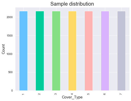
The target feature is homogeneously distributed amongst all 7 output classes.
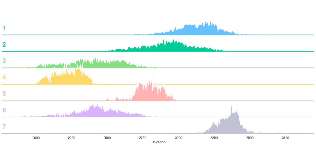
3.2. Elevation
plot_continuous_features(train,'Elevation','Cover_Type')
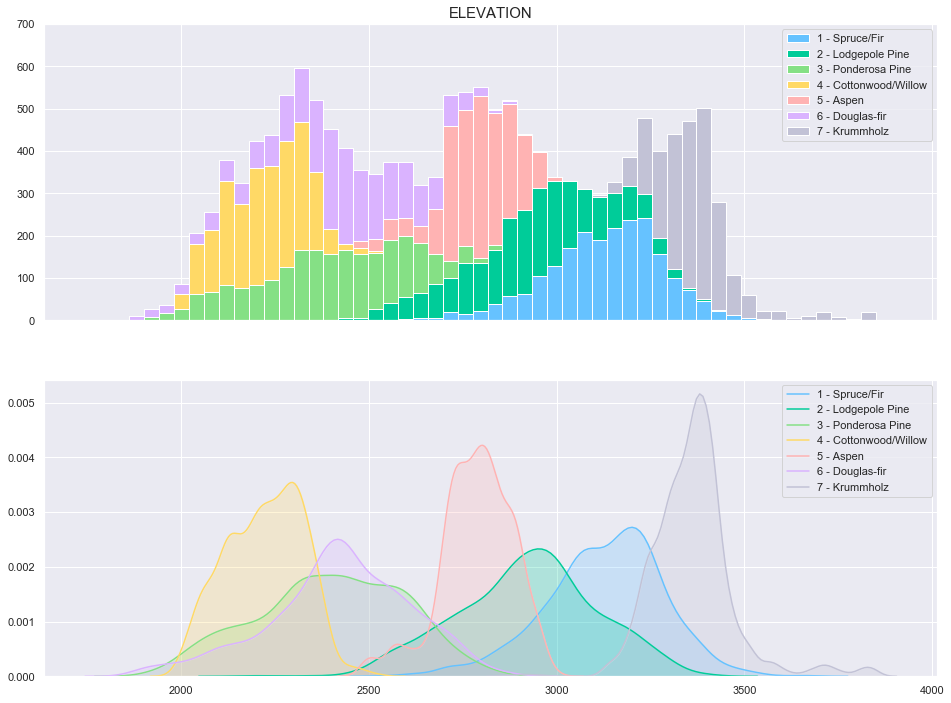
plot_3_plots('Elevation')
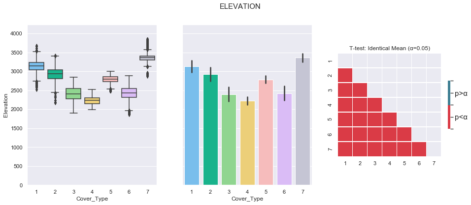
It can be observed from the above plots that the Cover Type can be fairly well separated using the elevation feature.
3.3. Aspect
plot_continuous_features(train,'Aspect','Cover_Type')
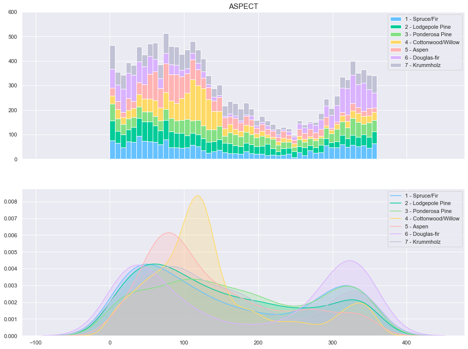
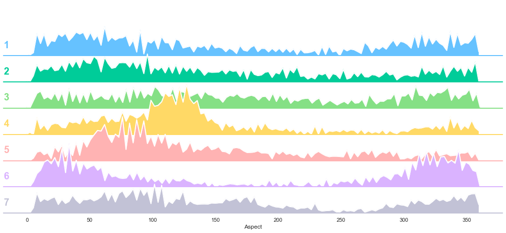
plot_3_plots('Aspect')
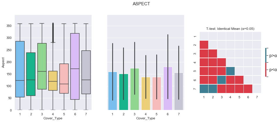
The Aspect feature does not appear to be a good class separator. Indeed, the t-test reveals several failures to reject the identical mean hypothesis (1-7, 2-7, 3-6, 4-6).
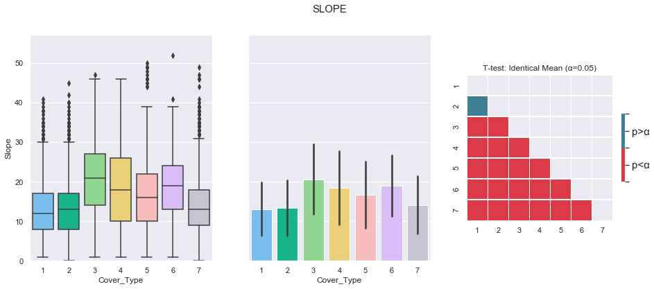
3.4. Slope
plot_continuous_features(train,'Slope','Cover_Type')
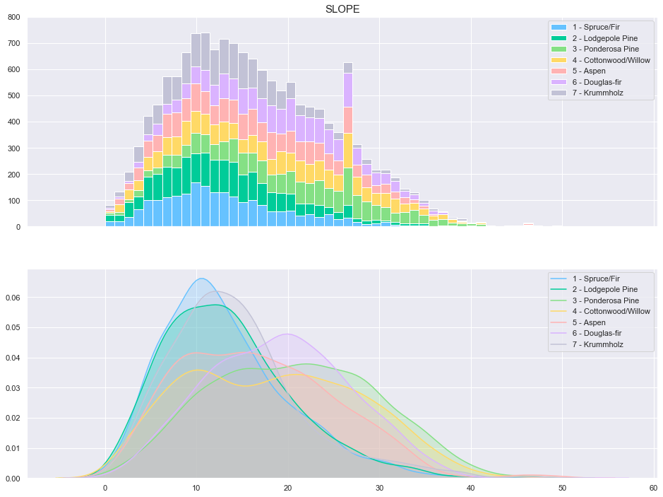
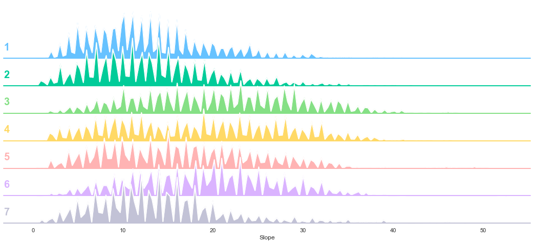
plot_3_plots('Slope')
3.5. Horizontal Distance To Hydrology
plot_continuous_features(train,'Horizontal_Distance_To_Hydrology','Cover_Type')
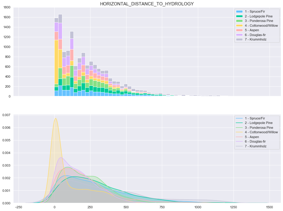
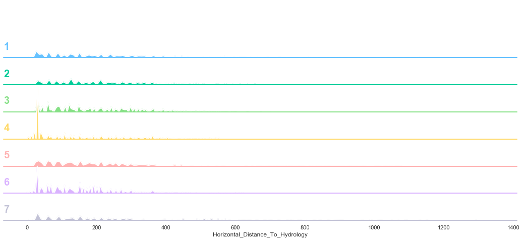
plot_3_plots('Horizontal_Distance_To_Hydrology')
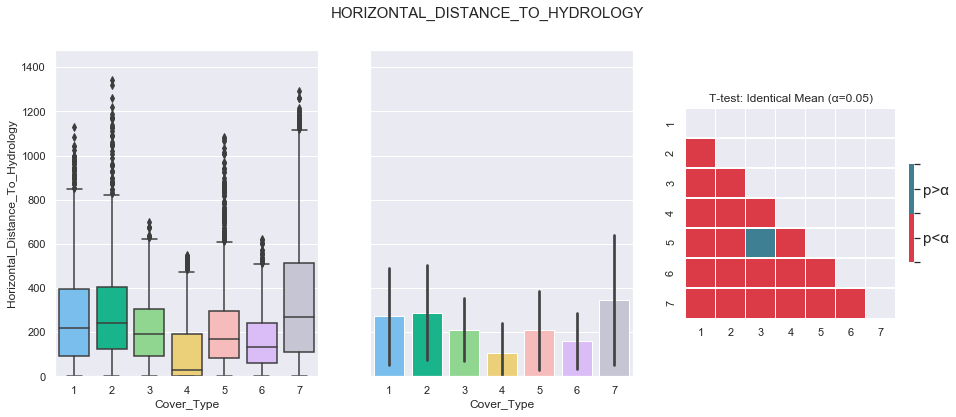
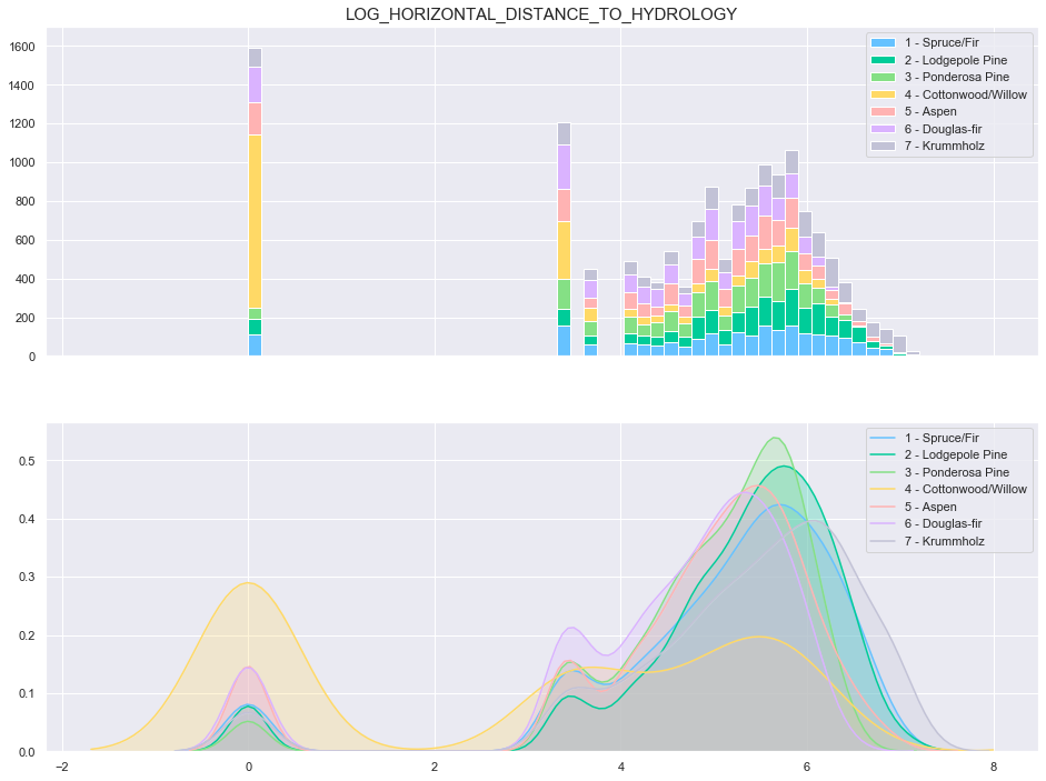
Based on the above plots, the data seems to be distributed according to a log distribution. In order to facilitate the classification, the log of the Horizontal Distance to Hydrology can be used.
train['log_Horizontal_Distance_To_Hydrology'] = train['Horizontal_Distance_To_Hydrology'].apply(lambda x: np.log(x) if x>0 else 0)
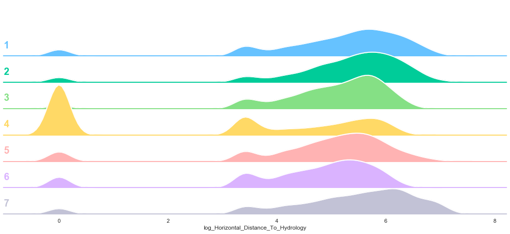
plot_continuous_features(train,'log_Horizontal_Distance_To_Hydrology','Cover_Type')
3.6. Vertical Distance To Hydrology
plot_continuous_features(train,'Vertical_Distance_To_Hydrology','Cover_Type')
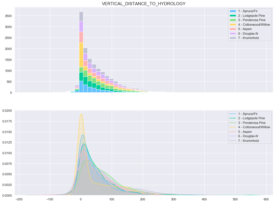
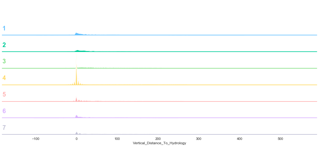
plot_3_plots('Vertical_Distance_To_Hydrology')
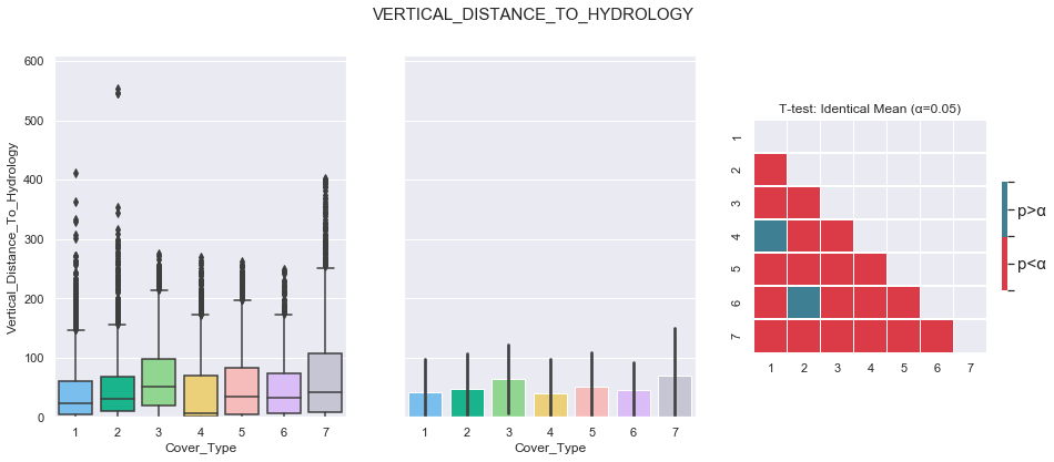
Similarly to the previous feature, the data seems to be distributed according to a log distribution. In order to facilitate the classification, the log of the Vertical Distance to Hydrology can be used.
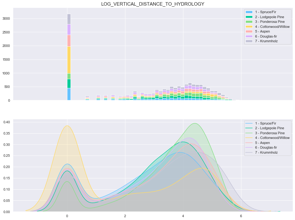
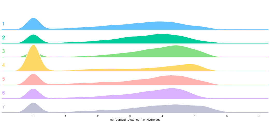
train['log_Vertical_Distance_To_Hydrology'] = train['Vertical_Distance_To_Hydrology'].apply(lambda x: np.log(x) if x>0 else 0)
plot_continuous_features(train,'log_Vertical_Distance_To_Hydrology','Cover_Type')
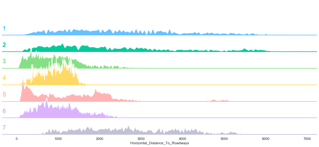
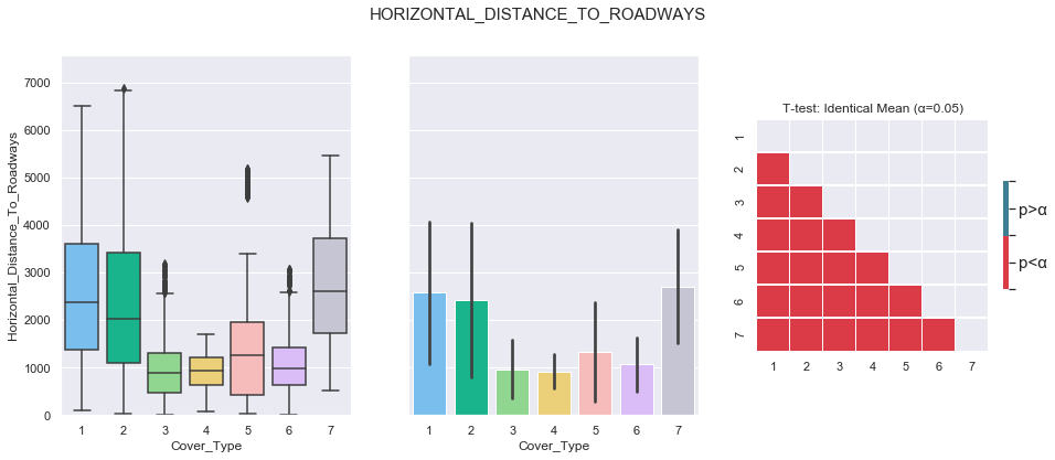
3.7. Horizontal Distance To Roadways
plot_continuous_features(train,'Horizontal_Distance_To_Roadways','Cover_Type')
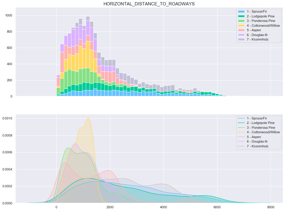
plot_3_plots('Horizontal_Distance_To_Roadways')
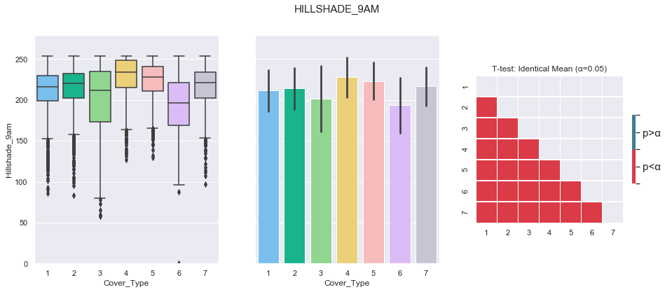
3.8. Hillshade 9am
plot_continuous_features(train,'Hillshade_9am','Cover_Type')
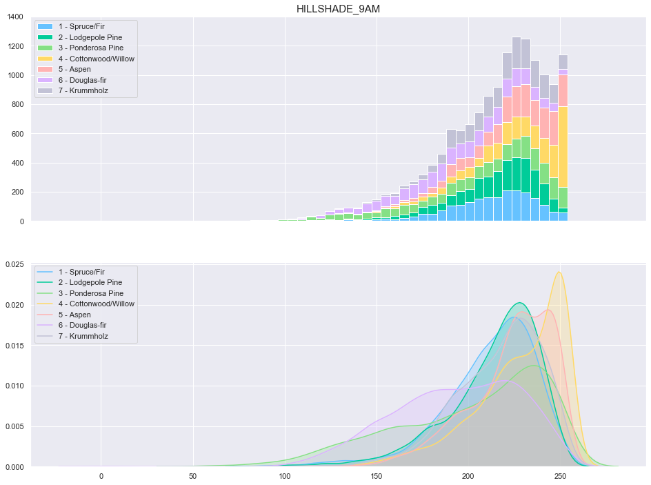
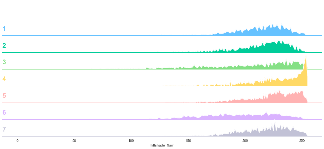
plot_3_plots('Hillshade_9am')
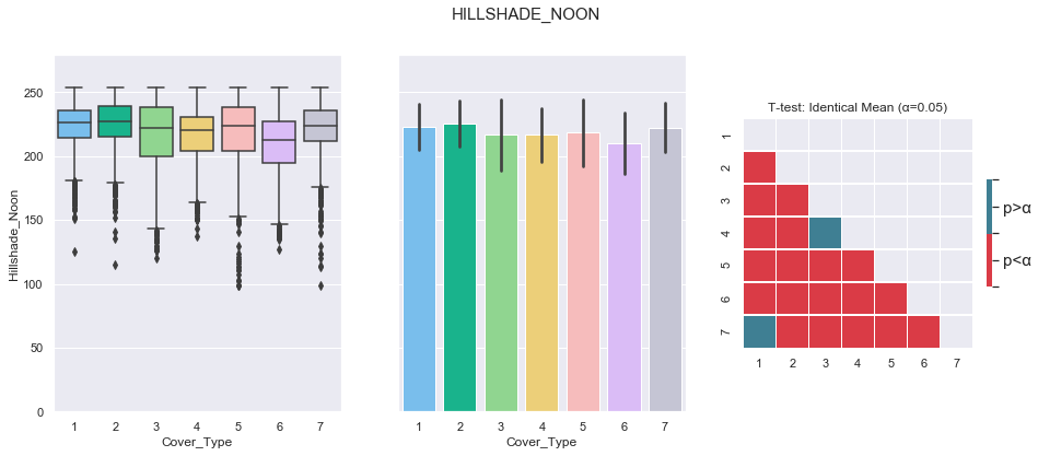
3.9. Hillshade Noon
plot_continuous_features(train,'Hillshade_Noon','Cover_Type')
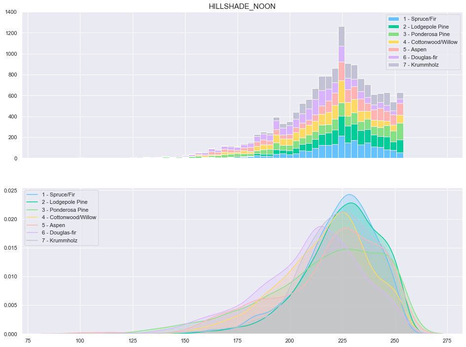
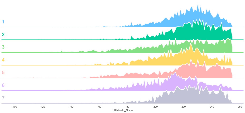
plot_3_plots('Hillshade_Noon')
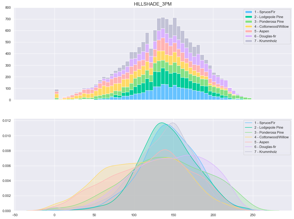
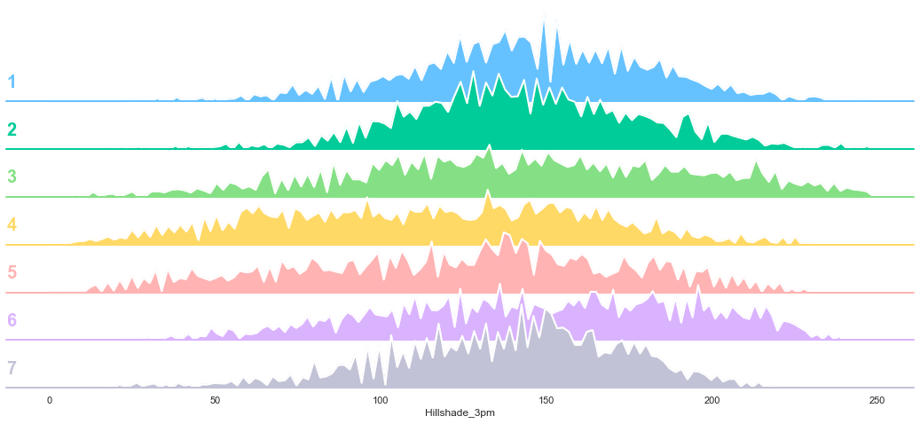
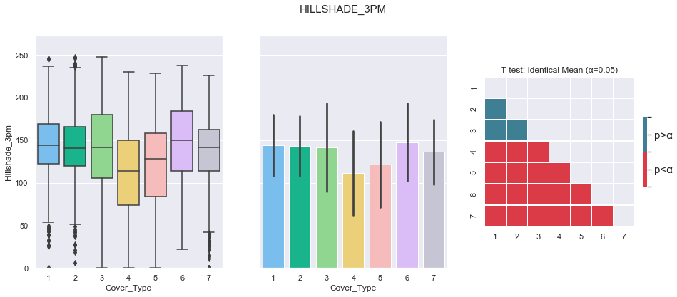
3.10. Hillshade 3 PM
plot_continuous_features(train,'Hillshade_3pm','Cover_Type')
plot_3_plots('Hillshade_3pm')
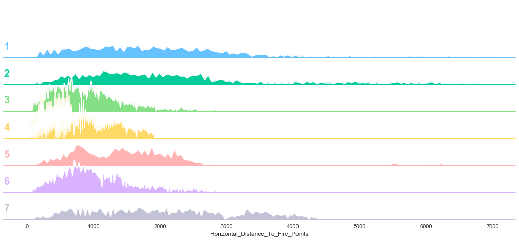
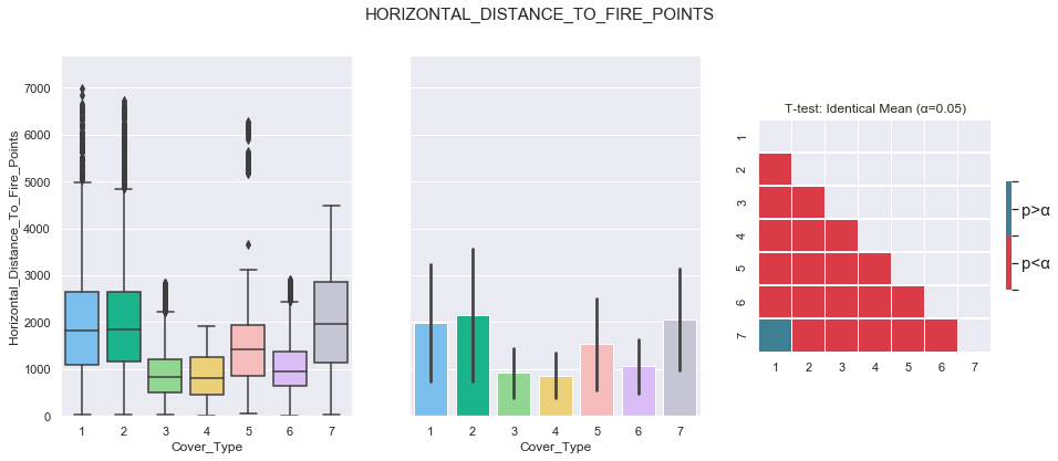
3.11. Horizontal Distance To Fire Points
plot_continuous_features(train,'Horizontal_Distance_To_Fire_Points','Cover_Type')
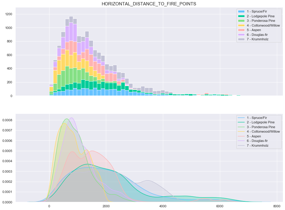
plot_3_plots('Horizontal_Distance_To_Fire_Points')
3.12. Wilderness Areas
plot_multiple_boolean_subclasses(train, 'Wilderness_Area', 'Cover_Type')
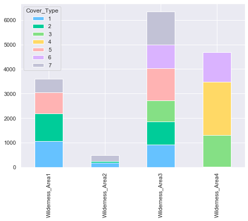
From the above plot, it can be seen that not every Cover Type is contained in each Wilderness Areas. For instance, the cover type “Ponderosa Pin” (3) is not present in the first two Wilderness Areas (Rawah Wilderness and Neota Wilderness Areas).
3.13. Soil Type
plot_multiple_boolean_subclasses(train, 'Soil_Type', 'Cover_Type')
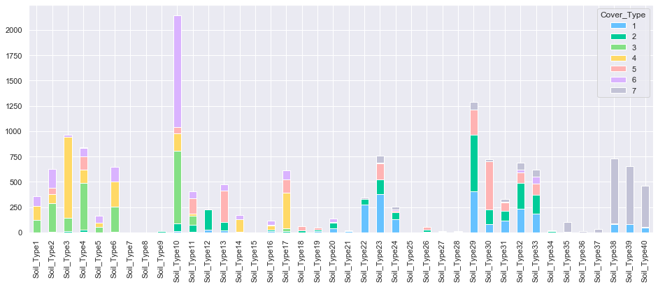
Several soil type do not contain any cover type. These features will be deleted.
# Data distribution
train.sum(axis=0).sort_values(ascending=True)[0:10]
Soil_Type15     0.0
Soil_Type7      0.0
Soil_Type25     1.0
Soil_Type8      1.0
Soil_Type28     9.0
Soil_Type36    10.0
Soil_Type9     10.0
Soil_Type27    15.0
Soil_Type21    16.0
Soil_Type34    22.0
dtype: float64
# drop empty soil types
def drop_empty_soil(train, test):
    '''drop the Soil_Type7 and Soil_Type15 features of train and test DataFrame.'''
    train = train.drop(['Soil_Type7', 'Soil_Type15'], axis=1)
    test = test.drop(['Soil_Type7', 'Soil_Type15'], axis=1)

    return train, test

# drop empty features
train, test = drop_empty_soil(train, test)
3.14. Feature Correlation
We produce a pair plot to evaluate the correlation between the target and the predictors.
# Compute the correlation matrix
corr = train[['Elevation', 'Aspect', 'Slope',
       'Horizontal_Distance_To_Hydrology', 'Vertical_Distance_To_Hydrology',
       'Horizontal_Distance_To_Roadways', 'Hillshade_9am', 'Hillshade_Noon',
       'Hillshade_3pm', 'Horizontal_Distance_To_Fire_Points']].corr()

# Generate a mask for the upper triangle
mask = np.zeros_like(corr, dtype=np.bool)
mask[np.triu_indices_from(mask)] = True

# Set up the matplotlib figure
f, ax = plt.subplots(figsize=(15, 13))

# Generate a custom diverging colormap
cmap = sns.diverging_palette(220, 10, as_cmap=True)

# Draw the heatmap with the mask and correct aspect ratio
g = sns.heatmap(corr, mask=mask, cmap=cmap, vmax=1.0,vmin=-1.0, center=0,annot=True,
            square=True, linewidths=.5, cbar_kws={"shrink": .3})
g.set_xticklabels(g.get_xticklabels(), rotation = 45, ha="right");
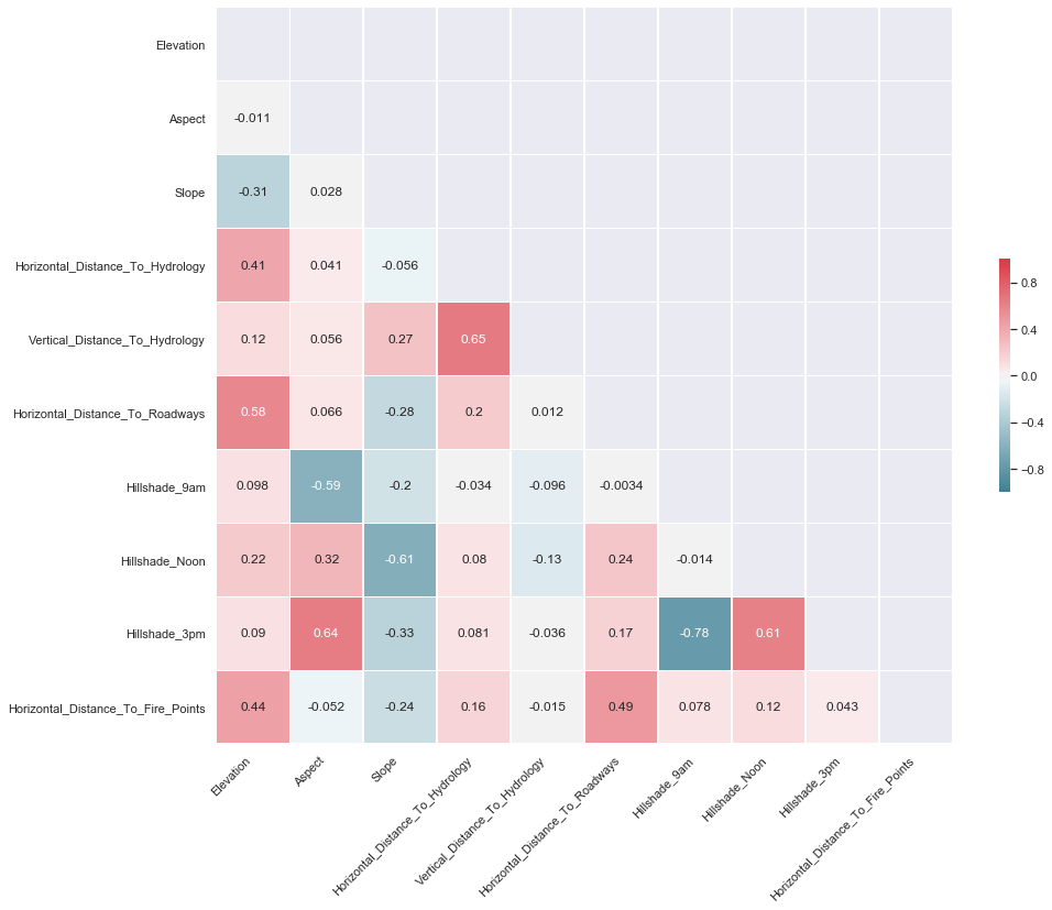
COMMENT: From the table above, we can notice the following large positive correlations:
- 0.65 between Vertical_Distance_To_Hydrology and Horizontal_Distance_To_Hydrology
- 0.64 between Hillshade_3pm and Aspect
- 0.61 between Hillshade_3pm and Hillshade_Noon
- 0.58 between Horizontal_Distance_To_Roadways and Elevation
From the table above, we can notice the following large negative correlations:
- -0.78 between Hillshade_3pm and Hillshade_9am
- -0.61 between Slope and Hillshade_Noon
- -0.59 between Hillshade_9am and Aspect
4. Feature Engineering
The following features will be added to the dataset:
| New Feature | Description |
|---|---|
| Hillshade_mean | mean of all three hillshade values |
| Euclidean_Distance_to_Hydrology | euclidean distance to hydrology (\(\sqrt{h^{2}+v{2}}\)) |
| Has_Soil_Type | is a soil type assigned to the record? |
| Cosine_Slope | cosine of slope |
| Sine_Slope | sine of slope |
| Slope_sq | slope squared |
| Elevation_sq | elevation squared |
| Aspect_sq | aspect squared |
| Horizontal_Distance_to_Hydrology_sq | horizontal distance to hydrology squared |
| Vertical_Distance_to_Hydrology_sq | vertical distance to hydrology squared |
| Horizontal_Distance_to_Roadways_sq | horizontal distance to roadways squared |
| Horizontal_Distance_to_Fire_Points_sq | horizontal distance to fire points squared |
| H_to_F_sum | Horizontal_Distance_to_Hydrology+Horizontal_Distance_to_Fire_Points |
| H_to_F_sub | Horizontal_Distance_to_Hydrology-Horizontal_Distance_to_Fire_Points |
| H_to_R_sum | Horizontal_Distance_to_Hydrology+Horizontal_Distance_to_Roadways |
| H_to_R_sub | Horizontal_Distance_to_Hydrology-Horizontal_Distance_to_Roadways |
| R_to_F_sum | Horizontal_Distance_to_Roadways+Horizontal_Distance_to_Fire_Points |
| R_to_F_sub | Horizontal_Distance_to_Roadways-Horizontal_Distance_to_Fire_Points |
| Slope_Hydrology | Vertical_Distance_to_Hydrology/Horizontal_Distance_to_Hydrology |
In order to process the data (train and test sets) in a consistent way, pipelines will be used. The pipeline consists of two branches: one for categorical features and the other for numerical features. Once the data going into each branch is processed, it will be re-combined into a single set.
-
Numerical Features:
a. Data selection: isolate numerical features from train or test set
b. Feature engineering: create new features based on numerical data
c. Scaler: scale data using standard scaler - Categorical Features:
a. Data selection: isolate categorical features from train or test set
b. Feature engineering: create new features based on categorical data - Union: combine the output of both pipelines
# load data
train = pd.read_csv('data/train.csv')
test = pd.read_csv('data/test.csv')

# save Id
train_ID = train['Id']
test_ID = test['Id']

# create X and y dataframe
X_train = train.drop(['Cover_Type'],axis=1).copy()
y_train = train['Cover_Type'].copy()
X_test = test.copy()

# drop iD
del X_train['Id']
del X_test['Id']
# isolate categorical and numerical feature
# different pipelines will be used
numerical_features = [
    'Elevation','Aspect','Slope','Horizontal_Distance_To_Hydrology',
    'Vertical_Distance_To_Hydrology','Horizontal_Distance_To_Roadways',
    'Hillshade_9am','Hillshade_Noon','Hillshade_3pm','Horizontal_Distance_To_Fire_Points']

catergorical_features = list(X_train.columns.difference(numerical_features))

new_numerical_features = [
    'log_Horizontal_Distance_To_Hydrology', 'log_Vertical_Distance_To_Hydrology',
    'Slope_sq', 'Elevation_sq', 'Aspect_sq', 'Horizontal_Distance_To_Hydrology_sq',
    'Vertical_Distance_To_Hydrology_sq','Horizontal_Distance_To_Roadways_sq',
    'Horizontal_Distance_To_Fire_Points_sq','Hillshade_mean','Euclidean_Distance_to_Hydrology',
    'Cosine_Slope','Sine_Slope','H_to_F_sum','H_to_F_sub','H_to_R_sum','H_to_R_sub','R_to_F_sum',
    'R_to_F_sub','Slope_Hydrology']

new_categorical_features = ['Has_Soil_Type']

full_feature_list_with = numerical_features+new_numerical_features+catergorical_features+new_categorical_features
full_feature_list_without = numerical_features+catergorical_features+new_categorical_features
# import scalers
from sklearn.preprocessing import MinMaxScaler, StandardScaler
from sklearn.pipeline import Pipeline
from sklearn.pipeline import FeatureUnion
class DataFrameSelector(BaseException, TransformerMixin):

    def __init__(self, attributes_names):
        self.attributes_names = attributes_names

    def fit(self, X, y=None):
        return self

    def transform(self, X, y=None):
        return X[self.attributes_names]
class NewNumericalFeatureGenerator(BaseEstimator, TransformerMixin):
    '''
    Generate new features on input dataframe.
    '''
    def __init__(self, add_new_features=True):
        self.add_new_features = add_new_features

    def fit(self, df, y=None):
        return self

    def transform(self, df, y=None):

        df_copy = df.copy()

        df_copy = df_copy.astype(np.float64)

        if self.add_new_features:

            # log features
            log_features = ['Horizontal_Distance_To_Hydrology', 'Vertical_Distance_To_Hydrology']

            for feature in log_features:
                df_copy['log_'+feature] = df_copy[feature].apply(lambda x: np.log(x) if x>0 else 0)

            # squared features
            squared_features = ['Slope', 'Elevation', 'Aspect', 'Horizontal_Distance_To_Hydrology',
                               'Vertical_Distance_To_Hydrology','Horizontal_Distance_To_Roadways',
                               'Horizontal_Distance_To_Fire_Points']

            for feature in squared_features:
                df_copy[feature+'_sq'] = df_copy[feature]**2

            # Hillshade_mean
            df_copy['Hillshade_mean'] = (df_copy['Hillshade_9am']+df_copy['Hillshade_Noon']+df_copy['Hillshade_3pm'])/3.

            # Euclidean_Distance_to_Hydrology
            df_copy['Euclidean_Distance_to_Hydrology'] = np.sqrt(df_copy['Horizontal_Distance_To_Hydrology_sq']+df_copy['Vertical_Distance_To_Hydrology_sq'])

            # Cosine_Slope
            df_copy['Cosine_Slope'] = np.cos(df_copy['Slope'] * np.pi / 180)

            # Sine_Slope
            df_copy['Sine_Slope'] = np.sin(df_copy['Slope'] * np.pi / 180)

            # H_to_F_sum
            df_copy['H_to_F_sum'] = np.abs(df_copy['Horizontal_Distance_To_Hydrology'] + df_copy['Horizontal_Distance_To_Fire_Points'])

            # H_to_F_sub
            df_copy['H_to_F_sub'] = np.abs(df_copy['Horizontal_Distance_To_Hydrology'] - df_copy['Horizontal_Distance_To_Fire_Points'])

            # H_to_R_sum
            df_copy['H_to_R_sum'] = np.abs(df_copy['Horizontal_Distance_To_Hydrology'] + df_copy['Horizontal_Distance_To_Roadways'])

            # H_to_R_sub
            df_copy['H_to_R_sub'] = np.abs(df_copy['Horizontal_Distance_To_Hydrology'] - df_copy['Horizontal_Distance_To_Roadways'])

            # R_to_F_sum
            df_copy['R_to_F_sum'] = np.abs(df_copy['Horizontal_Distance_To_Roadways'] + df_copy['Horizontal_Distance_To_Fire_Points'])

            # R_to_F_sub
            df_copy['R_to_F_sub'] = np.abs(df_copy['Horizontal_Distance_To_Roadways'] - df_copy['Horizontal_Distance_To_Fire_Points'])

            # Slope_Hydrology
            df_copy['Slope_Hydrology'] = df_copy['Vertical_Distance_To_Hydrology'] / df_copy['Horizontal_Distance_To_Hydrology']
            df_copy['Slope_Hydrology'] = df_copy['Slope_Hydrology'].map(lambda x: 0 if np.isnan(x) else x)

        return df_copy
class NewCategoricalFeatureGenerator(BaseEstimator, TransformerMixin):
    '''
    Generate new features on input dataframe.
    '''
    def __init__(self):
        pass

    def fit(self, df, y=None):
        return self

    def transform(self, df, y=None):

        df_copy = df.copy()

        # Has_Soil_Type
        soil_types = [x for x in df_copy.columns if 'Soil_Type' in x]
        df_copy['Has_Soil_Type'] = df_copy[soil_types].sum(axis=1)

        # return numpy array
        df_copy_values = df_copy.values

        return df_copy_values
class SpecialScaler(BaseEstimator, TransformerMixin):
    '''
    Standardize features
    '''
    def __init__(self, scaling_type='MinMax'):

        if scaling_type=='MinMax':
            self.scaler = MinMaxScaler()

        elif scaling_type=='StandardScaler':
            self.scaler = StandardScaler()

        else:
            self.scaler = None

    def fit(self, df, y=None):
        if self.scaler is None:
            pass
        else:
            self.scaler.fit(df)
        return self

    def transform(self, df):
        if self.scaler is None:
            return df.values
        else:
            return self.scaler.transform(df)
num_pipeline_with_new_features = Pipeline([
    ('selector',DataFrameSelector(numerical_features)),
    ('feature_adder',NewNumericalFeatureGenerator(add_new_features=True)),
    ('scaler',SpecialScaler(scaling_type='StandardScaler'))
])

num_pipeline_without_new_features = Pipeline([
    ('selector',DataFrameSelector(numerical_features)),
    ('feature_adder',NewNumericalFeatureGenerator(add_new_features=False)),
    ('scaler',SpecialScaler(scaling_type='StandardScaler'))
])


cat_pipeline = Pipeline([
    ('selector',DataFrameSelector(catergorical_features)),
    ('feature_adder',NewCategoricalFeatureGenerator()),
])

full_pipeline_with_new_features = FeatureUnion(transformer_list=[('num_pipeline',num_pipeline_with_new_features),
                                                                 ('cat_pipeline',cat_pipeline)])

full_pipeline_without_new_features = FeatureUnion(transformer_list=[('num_pipeline',num_pipeline_without_new_features),
                                                                    ('cat_pipeline',cat_pipeline)])
X_train_prepared_with = full_pipeline_with_new_features.fit_transform(X_train)
X_train_prepared_without = full_pipeline_without_new_features.fit_transform(X_train)
The new dataset contains a large number of attributes (76). In order to normalize our model, feature selection can be used to extract only the most important features. To do so, a simple Random Forest Classifier will be used.
from sklearn.ensemble import RandomForestClassifier
from sklearn.model_selection import GridSearchCV
# create model
forest_clf = RandomForestClassifier(random_state=42)

# create gridsearch
param_grid = {'n_estimators':[3,10,30,50,100],'max_features':[2,4,6,8],'max_depth':[3,5,10,15]}

# train model
grid_search_with = GridSearchCV(forest_clf,param_grid,cv=5,scoring='accuracy',n_jobs=4,verbose=2)
grid_search_with.fit(X_train_prepared_with, y_train)

grid_search_without = GridSearchCV(forest_clf,param_grid,cv=5,scoring='accuracy',n_jobs=4,verbose=2)
grid_search_without.fit(X_train_prepared_without, y_train)
Fitting 5 folds for each of 80 candidates, totalling 400 fits


[Parallel(n_jobs=4)]: Using backend LokyBackend with 4 concurrent workers.
[Parallel(n_jobs=4)]: Done  33 tasks      | elapsed:    4.1s
[Parallel(n_jobs=4)]: Done 154 tasks      | elapsed:   21.8s
[Parallel(n_jobs=4)]: Done 357 tasks      | elapsed:  1.2min
[Parallel(n_jobs=4)]: Done 400 out of 400 | elapsed:  1.5min finished


Fitting 5 folds for each of 80 candidates, totalling 400 fits


[Parallel(n_jobs=4)]: Using backend LokyBackend with 4 concurrent workers.
[Parallel(n_jobs=4)]: Done 128 tasks      | elapsed:    8.4s
[Parallel(n_jobs=4)]: Done 253 tasks      | elapsed:   20.3s
[Parallel(n_jobs=4)]: Done 400 out of 400 | elapsed:   47.1s finished


GridSearchCV(cv=5, error_score='raise-deprecating',
             estimator=RandomForestClassifier(bootstrap=True, class_weight=None,
                                              criterion='gini', max_depth=None,
                                              max_features='auto',
                                              max_leaf_nodes=None,
                                              min_impurity_decrease=0.0,
                                              min_impurity_split=None,
                                              min_samples_leaf=1,
                                              min_samples_split=2,
                                              min_weight_fraction_leaf=0.0,
                                              n_estimators='warn', n_jobs=None,
                                              oob_score=False, random_state=42,
                                              verbose=0, warm_start=False),
             iid='warn', n_jobs=4,
             param_grid={'max_depth': [3, 5, 10, 15],
                         'max_features': [2, 4, 6, 8],
                         'n_estimators': [3, 10, 30, 50, 100]},
             pre_dispatch='2*n_jobs', refit=True, return_train_score=False,
             scoring='accuracy', verbose=2)
print("Best accuracy with new features",grid_search_with.best_score_)
print("Best accuracy without new features",grid_search_without.best_score_)
Best accuracy with new features 0.7851190476190476
Best accuracy without new features 0.7618386243386244
feature_importances_with = grid_search_with.best_estimator_.feature_importances_

for ix,item in enumerate(sorted(zip(feature_importances_with,full_feature_list_with),reverse=True)):
    print(ix+1, item)
1 (0.14152351076150732, 'Elevation')
2 (0.13190518916873342, 'Elevation_sq')
3 (0.03878816856795683, 'R_to_F_sum')
4 (0.03687988835737898, 'Wilderness_Area4')
5 (0.03465820030896246, 'H_to_R_sub')
6 (0.02969575956564049, 'Horizontal_Distance_To_Roadways')
7 (0.028719686262350896, 'H_to_R_sum')
8 (0.028414939013321355, 'Horizontal_Distance_To_Roadways_sq')
9 (0.025056946923004707, 'R_to_F_sub')
10 (0.023834760808291177, 'H_to_F_sum')
11 (0.02263890186894855, 'Hillshade_9am')
12 (0.022235681492061888, 'Horizontal_Distance_To_Fire_Points')
13 (0.020816744245214534, 'Horizontal_Distance_To_Fire_Points_sq')
14 (0.020300429050862795, 'Euclidean_Distance_to_Hydrology')
15 (0.02020020125477723, 'Aspect')
16 (0.01966048192263614, 'H_to_F_sub')
17 (0.01944452869164485, 'Aspect_sq')
18 (0.018757557523025766, 'Soil_Type10')
19 (0.017981809544327057, 'Horizontal_Distance_To_Hydrology_sq')
20 (0.01681290363696822, 'Vertical_Distance_To_Hydrology_sq')
21 (0.01628750794156562, 'Hillshade_3pm')
22 (0.015767908168667726, 'Soil_Type3')
23 (0.015684408039363464, 'log_Horizontal_Distance_To_Hydrology')
24 (0.015621261267752283, 'Horizontal_Distance_To_Hydrology')
25 (0.015577123262199837, 'Wilderness_Area3')
26 (0.015336705888016116, 'Wilderness_Area1')
27 (0.015086774235711094, 'Hillshade_Noon')
28 (0.014486586781480938, 'Soil_Type38')
29 (0.01425128617291883, 'Hillshade_mean')
30 (0.013858095606874144, 'Slope_Hydrology')
31 (0.013770929149894306, 'Vertical_Distance_To_Hydrology')
32 (0.013590421450373293, 'Soil_Type39')
33 (0.011584893055557866, 'log_Vertical_Distance_To_Hydrology')
34 (0.00883439889425353, 'Cosine_Slope')
35 (0.008824731678667782, 'Sine_Slope')
36 (0.008519215091788636, 'Slope')
37 (0.008406001964489292, 'Soil_Type4')
38 (0.008049744667644264, 'Slope_sq')
39 (0.007418427316254516, 'Soil_Type40')
40 (0.00591836799042853, 'Soil_Type30')
41 (0.003449767700896693, 'Soil_Type13')
42 (0.003026236704389329, 'Wilderness_Area2')
43 (0.002917783790374529, 'Soil_Type12')
44 (0.002792952520826473, 'Soil_Type29')
45 (0.0027696099299623278, 'Soil_Type32')
46 (0.0027157440327077276, 'Soil_Type2')
47 (0.0027039817262601417, 'Soil_Type22')
48 (0.002654504572087974, 'Soil_Type23')
49 (0.0019415364596016252, 'Soil_Type17')
50 (0.0016143585426425708, 'Soil_Type33')
51 (0.0012767757230445415, 'Soil_Type6')
52 (0.0009590220884099596, 'Soil_Type11')
53 (0.0009310613728797029, 'Soil_Type35')
54 (0.000785856673361728, 'Soil_Type31')
55 (0.0007823089137053381, 'Soil_Type24')
56 (0.0007530883967865013, 'Soil_Type1')
57 (0.0006799707571842439, 'Soil_Type20')
58 (0.0005747015598076818, 'Soil_Type5')
59 (0.0004453989768105188, 'Soil_Type16')
60 (0.0002218366821015433, 'Soil_Type18')
61 (0.00018435985478080187, 'Soil_Type14')
62 (0.00014059895771458805, 'Soil_Type37')
63 (0.0001318831735853356, 'Soil_Type26')
64 (9.608551995037555e-05, 'Soil_Type19')
65 (5.027960141285551e-05, 'Soil_Type34')
66 (4.949345221571494e-05, 'Soil_Type28')
67 (4.555758972482114e-05, 'Soil_Type27')
68 (4.371425550097232e-05, 'Soil_Type21')
69 (3.9161118007753776e-05, 'Soil_Type9')
70 (1.7843910376931404e-05, 'Soil_Type36')
71 (3.43710410880248e-06, 'Soil_Type25')
72 (1.0747263197141472e-08, 'Soil_Type8')
73 (0.0, 'Soil_Type7')
74 (0.0, 'Soil_Type15')
75 (0.0, 'Has_Soil_Type')
feature_importances_without = grid_search_without.best_estimator_.feature_importances_

for ix,item in enumerate(sorted(zip(feature_importances_without,full_feature_list_without),reverse=True)):
    print(ix+1, item)
1 (0.25878829585756613, 'Elevation')
2 (0.08698109411500367, 'Horizontal_Distance_To_Roadways')
3 (0.06334081721558939, 'Horizontal_Distance_To_Fire_Points')
4 (0.05736072766500386, 'Wilderness_Area4')
5 (0.05640103379348544, 'Horizontal_Distance_To_Hydrology')
6 (0.045080251148035336, 'Hillshade_9am')
7 (0.043516585043468704, 'Vertical_Distance_To_Hydrology')
8 (0.04002124407977922, 'Aspect')
9 (0.03817656728870067, 'Hillshade_3pm')
10 (0.03472020682173347, 'Hillshade_Noon')
11 (0.027799274938067668, 'Soil_Type10')
12 (0.02573161368161303, 'Slope')
13 (0.02450273362314368, 'Soil_Type39')
14 (0.024484916872244165, 'Soil_Type38')
15 (0.021348381588154094, 'Wilderness_Area3')
16 (0.020457233904003884, 'Wilderness_Area1')
17 (0.020147880229841632, 'Soil_Type3')
18 (0.0144625025231886, 'Soil_Type4')
19 (0.01133349335971847, 'Soil_Type40')
20 (0.00910708906663545, 'Soil_Type30')
21 (0.007926063722480137, 'Soil_Type22')
22 (0.00722141237917537, 'Soil_Type13')
23 (0.0064434542330762505, 'Soil_Type17')
24 (0.006077001190013304, 'Soil_Type29')
25 (0.005918225908316521, 'Soil_Type2')
26 (0.00535686144733342, 'Soil_Type12')
27 (0.0052671046186313995, 'Wilderness_Area2')
28 (0.005136083279655753, 'Soil_Type23')
29 (0.0043006374729556394, 'Soil_Type32')
30 (0.002987245513505226, 'Soil_Type33')
31 (0.002895173751792928, 'Soil_Type6')
32 (0.002441118962703501, 'Soil_Type11')
33 (0.0024339839669552097, 'Soil_Type35')
34 (0.0018534233806203665, 'Soil_Type24')
35 (0.0018524652699843077, 'Soil_Type1')
36 (0.001434765633805951, 'Soil_Type31')
37 (0.0012583713883418176, 'Soil_Type5')
38 (0.0011774069004786391, 'Soil_Type20')
39 (0.0008610774455624859, 'Soil_Type18')
40 (0.0007952791538882718, 'Soil_Type14')
41 (0.0007862567472032722, 'Soil_Type16')
42 (0.000710748968022875, 'Soil_Type37')
43 (0.0002163889962338194, 'Soil_Type26')
44 (0.00020074267666505787, 'Soil_Type19')
45 (0.00016198783895200196, 'Soil_Type34')
46 (0.00011485179619529112, 'Soil_Type21')
47 (0.00010892953211897586, 'Soil_Type27')
48 (0.00010745256745145929, 'Soil_Type9')
49 (8.916452586339112e-05, 'Soil_Type36')
50 (7.186961540098499e-05, 'Soil_Type28')
51 (3.003375547567885e-05, 'Soil_Type25')
52 (2.4745461639670084e-06, 'Soil_Type8')
53 (0.0, 'Soil_Type7')
54 (0.0, 'Soil_Type15')
55 (0.0, 'Has_Soil_Type')
The above list shows several feature which do no impact the model (Soil_Type8, 7 and 15). Therefore, in the final tuning of our model, the number of selected features will be integreted as a tunable hyperparameter.
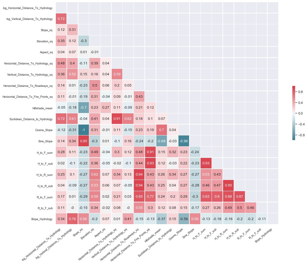
X_train_new_features = NewNumericalFeatureGenerator(add_new_features=True).fit_transform(X_train)
# Compute the correlation matrix
corr = X_train_new_features[new_numerical_features].corr()
corr = np.around(corr, decimals=2)

# Generate a mask for the upper triangle
mask = np.zeros_like(corr, dtype=np.bool)
mask[np.triu_indices_from(mask)] = True

# Set up the matplotlib figure
f, ax = plt.subplots(figsize=(16, 16))

# Generate a custom diverging colormap
cmap = sns.diverging_palette(220, 10, as_cmap=True)

# Draw the heatmap with the mask and correct aspect ratio
g = sns.heatmap(corr, mask=mask, cmap=cmap, vmax=1.0,vmin=-1.0, center=0,annot=True,
            square=True, linewidths=.5, cbar_kws={"shrink": .2})
g.set_xticklabels(g.get_xticklabels(), rotation = 40, fontsize = 9, ha='right')
g.set_yticklabels(g.get_yticklabels(), fontsize = 9);
# add feature selection to grid search
def indices_of_top_k(arr, k):
    return np.sort(np.argpartition(np.array(arr),-k)[-k:])

class TopFeatureSelector(BaseEstimator, TransformerMixin):
    '''Select the k best feature from dataset'''

    def __init__(self, feature_importances, k):
        self.feature_importances = feature_importances
        self.k = k

    def fit(self, X, y=None):
        self.feature_indices_ = indices_of_top_k(self.feature_importances, self.k)
        return self

    def transform(self, X):
        return X[:, self.feature_indices_]
# first example
k = 45
# pipeline
preparation_and_feature_selection_pipeline_with = Pipeline([
    ('preparation',full_pipeline_with_new_features),
    ('feature_selection',TopFeatureSelector(feature_importances_with,k))
])

preparation_and_feature_selection_pipeline_without = Pipeline([
    ('preparation',full_pipeline_without_new_features),
    ('feature_selection',TopFeatureSelector(feature_importances_without,k))
])
preparation_and_feature_selection_pipeline_with.fit(X_train)
preparation_and_feature_selection_pipeline_without.fit(X_train)

X_train_prepared_with = preparation_and_feature_selection_pipeline_with.transform(X_train)
X_train_prepared_without = preparation_and_feature_selection_pipeline_without.transform(X_train)
5. Models
The following classifiers are used to predict the forest types:
- Logistic Regression (Classification)
- K-Nearest Neighbors
- Support Vector Machines
- Gaussian Naive Bayes
- Decision Tree Classifier
- Bagging
- Random Forest Classifier
- Gradient Boosting Classifier
- Linear Discriminant Analysis
- NN
- Adaboost
- Extra Trees
# import modules
# Models
from sklearn.tree import DecisionTreeClassifier, DecisionTreeRegressor
from sklearn.model_selection import cross_val_score,GridSearchCV, StratifiedKFold, train_test_split
from sklearn.naive_bayes import GaussianNB
from sklearn.tree import DecisionTreeClassifier
from sklearn.ensemble import RandomForestClassifier, GradientBoostingClassifier, BaggingClassifier
from sklearn.svm import SVC
from sklearn.preprocessing import StandardScaler
from sklearn.linear_model import LogisticRegression, SGDClassifier
from sklearn.neighbors import KNeighborsClassifier
from sklearn.discriminant_analysis import LinearDiscriminantAnalysis
from sklearn.neural_network import MLPClassifier
from sklearn.ensemble import AdaBoostClassifier, VotingClassifier, ExtraTreesClassifier

from xgboost import XGBClassifier

# cross validation
from sklearn.model_selection import train_test_split, cross_val_score
from sklearn.metrics import accuracy_score
# cross validate model with Kfold stratified cross val
kfold = StratifiedKFold(n_splits=10)
# random state used for all models
random_state = 42
# store models in list
classifiers_list = []

classifiers_list.append(LogisticRegression(random_state=random_state))
classifiers_list.append(KNeighborsClassifier())
classifiers_list.append(SVC(random_state=random_state))
classifiers_list.append(GaussianNB())
classifiers_list.append(DecisionTreeClassifier(random_state=random_state))
classifiers_list.append(BaggingClassifier(random_state=random_state))
classifiers_list.append(RandomForestClassifier(random_state=random_state))
classifiers_list.append(GradientBoostingClassifier(random_state=random_state))
classifiers_list.append(LinearDiscriminantAnalysis())
classifiers_list.append(MLPClassifier(random_state=random_state))
classifiers_list.append(AdaBoostClassifier(DecisionTreeClassifier(random_state=random_state),random_state=random_state))
classifiers_list.append(ExtraTreesClassifier(random_state=random_state))
classifiers_list.append(SGDClassifier(random_state=random_state))
classifiers_list.append(XGBClassifier(random_state=random_state))

# store cv results in list
cv_results_list = []
cv_means_list = []
cv_std_list = []

# perform cross-validation
for clf in classifiers_list:
    cv_results_list.append(cross_val_score(clf,
                                           X_train_prepared_with,
                                           y_train,
                                           scoring = "accuracy",
                                           cv = kfold,
                                           n_jobs=4))

    cv_results_list.append(cross_val_score(clf,
                                           X_train_prepared_without,
                                           y_train,
                                           scoring = "accuracy",
                                           cv = kfold,
                                           n_jobs=4))

    print("Training {}: Done".format(type(clf).__name__))

# store mean and std accuracy
for cv_result in cv_results_list:
    cv_means_list.append(cv_result.mean())
    cv_std_list.append(cv_result.std())

cv_res_df = pd.DataFrame({"CrossValMeans":cv_means_list,
                          "CrossValerrors": cv_std_list,
                          "Algorithm":["LogReg_with","LogReg","KNN_with","KNN","SVC_with","SVC",
                                       "GaussianNB_with","GaussianNB","DecisionTree_with","DecisionTree",
                                       "Bagging_with","Bagging","RdmForest_with","RdmForest",
                                       "GradientBoost_with","GradientBoost","LDA_with","LDA",
                                       "NN_with","NN","AdaBoost_with","AdaBoost",
                                       "ExtraTrees","ExtraTrees_with",'SGDC','SGDC_with','XGBC_with','XGBC']})

cv_res_df = cv_res_df.sort_values(by='CrossValMeans',ascending=False)
Training LogisticRegression: Done
Training KNeighborsClassifier: Done
Training SVC: Done
Training GaussianNB: Done
Training DecisionTreeClassifier: Done
Training BaggingClassifier: Done
Training RandomForestClassifier: Done
Training GradientBoostingClassifier: Done
Training LinearDiscriminantAnalysis: Done
Training MLPClassifier: Done
Training AdaBoostClassifier: Done
Training ExtraTreesClassifier: Done
Training SGDClassifier: Done
Training XGBClassifier: Done
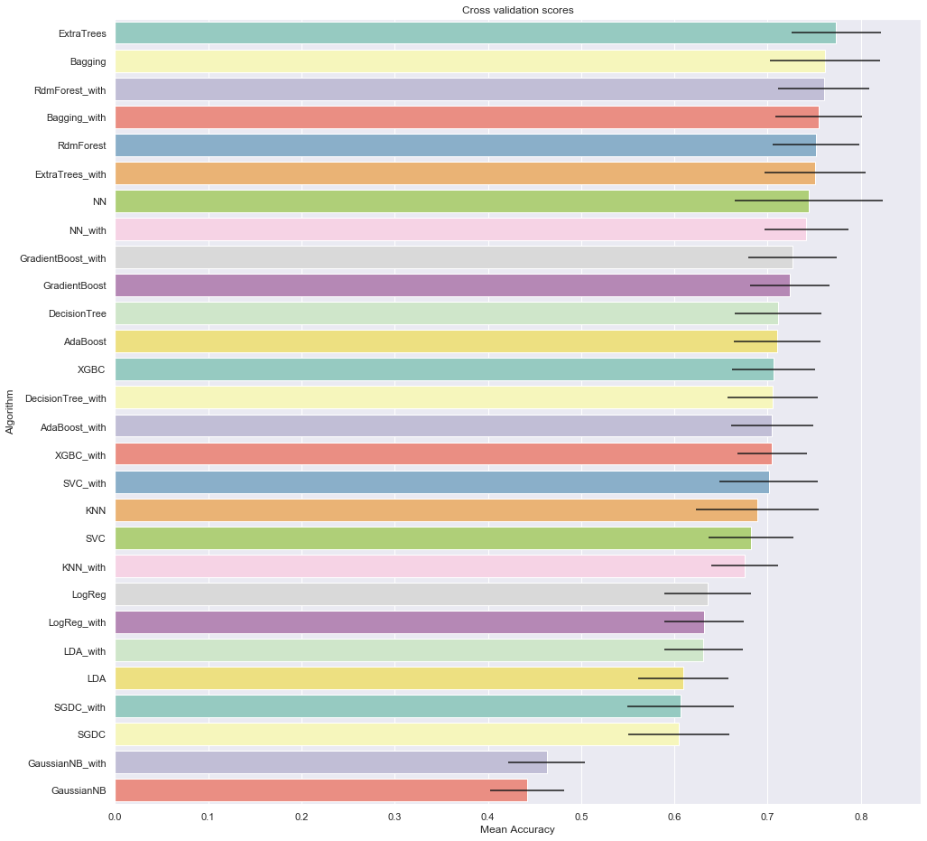
# plot results
fig, ax = plt.subplots(figsize=(16,16))
g = sns.barplot("CrossValMeans",
                "Algorithm",
                data = cv_res_df,
                palette="Set3",
                orient = "h", ax=ax,
                **{'xerr':cv_std_list})
g.set_xlabel("Mean Accuracy")
g = g.set_title("Cross validation scores")
from sklearn.model_selection import GridSearchCV
prepare_select_and_predict_pipeline = Pipeline([
    ('preparation',full_pipeline_with_new_features),
    ('feature_selection',TopFeatureSelector(feature_importances_with,k)),
    ('extra_tree',ExtraTreesClassifier(random_state=42))
])
extra_tree_clf = ExtraTreesClassifier(random_state=42)

param_grid = [{'extra_tree__n_estimators':[50,100,150],
               'extra_tree__criterion':['gini','entropy'],
               'extra_tree__max_depth':[3,5,10,15,20],
               'extra_tree__min_samples_split':[2,3,5],
               'extra_tree__min_samples_leaf':[2,3,5],
               'extra_tree__max_features':['auto',None],
               'feature_selection__feature_importances':[feature_importances_with],
               'feature_selection__k':[10, 20, 30, 45],
               'preparation__num_pipeline__feature_adder__add_new_features':[True]},
              {'extra_tree__n_estimators':[50,100,150],
               'extra_tree__criterion':['gini','entropy'],
               'extra_tree__max_depth':[3,5,10,15,20],
               'extra_tree__min_samples_split':[2,3,5],
               'extra_tree__min_samples_leaf':[2,3,5],
               'extra_tree__max_features':['auto',None],
               'feature_selection__feature_importances':[feature_importances_without],
               'feature_selection__k':[10, 20, 30, 45],
               'preparation__num_pipeline__feature_adder__add_new_features':[False]}
             ]
grid_search_pipeline = GridSearchCV(prepare_select_and_predict_pipeline,param_grid,cv=5,scoring='accuracy',verbose=1,n_jobs=4)
grid_search_pipeline.fit(X_train, y_train)
Fitting 5 folds for each of 4320 candidates, totalling 21600 fits


[Parallel(n_jobs=4)]: Using backend LokyBackend with 4 concurrent workers.
[Parallel(n_jobs=4)]: Done  42 tasks      | elapsed:   15.5s
[Parallel(n_jobs=4)]: Done 192 tasks      | elapsed:   42.9s
[Parallel(n_jobs=4)]: Done 442 tasks      | elapsed:  1.4min
[Parallel(n_jobs=4)]: Done 792 tasks      | elapsed:  3.2min
[Parallel(n_jobs=4)]: Done 1242 tasks      | elapsed:  5.9min
[Parallel(n_jobs=4)]: Done 1792 tasks      | elapsed:  8.5min
[Parallel(n_jobs=4)]: Done 2442 tasks      | elapsed: 14.0min
[Parallel(n_jobs=4)]: Done 3192 tasks      | elapsed: 24.8min
[Parallel(n_jobs=4)]: Done 4042 tasks      | elapsed: 34.1min
[Parallel(n_jobs=4)]: Done 4992 tasks      | elapsed: 50.1min
[Parallel(n_jobs=4)]: Done 6042 tasks      | elapsed: 59.8min
[Parallel(n_jobs=4)]: Done 7192 tasks      | elapsed: 65.2min
[Parallel(n_jobs=4)]: Done 8442 tasks      | elapsed: 75.0min
[Parallel(n_jobs=4)]: Done 9792 tasks      | elapsed: 91.2min
[Parallel(n_jobs=4)]: Done 11242 tasks      | elapsed: 105.9min
[Parallel(n_jobs=4)]: Done 12792 tasks      | elapsed: 111.4min
[Parallel(n_jobs=4)]: Done 14442 tasks      | elapsed: 121.0min
[Parallel(n_jobs=4)]: Done 16192 tasks      | elapsed: 138.0min
[Parallel(n_jobs=4)]: Done 18042 tasks      | elapsed: 143.8min
[Parallel(n_jobs=4)]: Done 19992 tasks      | elapsed: 155.7min
[Parallel(n_jobs=4)]: Done 21600 out of 21600 | elapsed: 172.5min finished


GridSearchCV(cv=5, error_score='raise-deprecating',
             estimator=Pipeline(memory=None,
                                steps=[('preparation',
                                        FeatureUnion(n_jobs=None,
                                                     transformer_list=[('num_pipeline',
                                                                        Pipeline(memory=None,
                                                                                 steps=[('selector',
                                                                                         DataFrameSelector(['Elevation', 'Aspect', 'Slope', 'Horizontal_Distance_To_Hydrology', 'Vertical_Distance_To_Hydrology', 'Horizontal_Distance_To_Roadways...
       1.13334934e-02, 1.25837139e-03, 2.89517375e-03, 0.00000000e+00,
       2.47454616e-06, 1.07452567e-04, 2.04572339e-02, 5.26710462e-03,
       2.13483816e-02, 5.73607277e-02, 0.00000000e+00])],
                          'feature_selection__k': [10, 20, 30, 45],
                          'preparation__num_pipeline__feature_adder__add_new_features': [False]}],
             pre_dispatch='2*n_jobs', refit=True, return_train_score=False,
             scoring='accuracy', verbose=1)
grid_search_pipeline.best_score_
0.8001322751322751
grid_search_pipeline.best_params_
{'extra_tree__criterion': 'entropy',
 'extra_tree__max_depth': 20,
 'extra_tree__max_features': None,
 'extra_tree__min_samples_leaf': 2,
 'extra_tree__min_samples_split': 2,
 'extra_tree__n_estimators': 100,
 'feature_selection__feature_importances': array([1.41523511e-01, 2.02002013e-02, 8.51921509e-03, 1.56212613e-02,
        1.37709291e-02, 2.96957596e-02, 2.26389019e-02, 1.50867742e-02,
        1.62875079e-02, 2.22356815e-02, 1.56844080e-02, 1.15848931e-02,
        8.04974467e-03, 1.31905189e-01, 1.94445287e-02, 1.79818095e-02,
        1.68129036e-02, 2.84149390e-02, 2.08167442e-02, 1.42512862e-02,
        2.03004291e-02, 8.83439889e-03, 8.82473168e-03, 2.38347608e-02,
        1.96604819e-02, 2.87196863e-02, 3.46582003e-02, 3.87881686e-02,
        2.50569469e-02, 1.38580956e-02, 7.53088397e-04, 1.87575575e-02,
        9.59022088e-04, 2.91778379e-03, 3.44976770e-03, 1.84359855e-04,
        0.00000000e+00, 4.45398977e-04, 1.94153646e-03, 2.21836682e-04,
        9.60855200e-05, 2.71574403e-03, 6.79970757e-04, 4.37142555e-05,
        2.70398173e-03, 2.65450457e-03, 7.82308914e-04, 3.43710411e-06,
        1.31883174e-04, 4.55575897e-05, 4.94934522e-05, 2.79295252e-03,
        1.57679082e-02, 5.91836799e-03, 7.85856673e-04, 2.76960993e-03,
        1.61435854e-03, 5.02796014e-05, 9.31061373e-04, 1.78439104e-05,
        1.40598958e-04, 1.44865868e-02, 1.35904215e-02, 8.40600196e-03,
        7.41842732e-03, 5.74701560e-04, 1.27677572e-03, 0.00000000e+00,
        1.07472632e-08, 3.91611180e-05, 1.53367059e-02, 3.02623670e-03,
        1.55771233e-02, 3.68798884e-02, 0.00000000e+00]),
 'feature_selection__k': 30,
 'preparation__num_pipeline__feature_adder__add_new_features': True}
6. Submission
submission_pipeline = Pipeline([
    ('preparation',full_pipeline_with_new_features),
    ('feature_selection',TopFeatureSelector(feature_importances_with,30))
])

X_train_prep = submission_pipeline.fit_transform(X_train)
final_model = ExtraTreesClassifier(random_state=42, criterion='entropy',
max_depth=20,
max_features=None,
min_samples_leaf=2,
min_samples_split= 2,
n_estimators=100)

final_model.fit(X_train_prep,y_train)
ExtraTreesClassifier(bootstrap=False, class_weight=None, criterion='entropy',
                     max_depth=20, max_features=None, max_leaf_nodes=None,
                     min_impurity_decrease=0.0, min_impurity_split=None,
                     min_samples_leaf=2, min_samples_split=2,
                     min_weight_fraction_leaf=0.0, n_estimators=100,
                     n_jobs=None, oob_score=False, random_state=42, verbose=0,
                     warm_start=False)
X_test_prep = submission_pipeline.transform(X_test)
# make prediction on test set
y_test_pred = final_model.predict(X_test_prep).astype(int)
# generate submission file
submission_df = pd.DataFrame({'Id': test_ID,
                            'Cover_Type': y_test_pred})
submission_df.to_csv("extra_tree_full_pipe.csv", index=False)
Conclusion: The accuracy on the test set is computed by Kaggle. Our model obtained an accuracy of 77%. This approximately ranks in the top 10% of the competition.