Kaggle: Housing Price Predictions (Top 5%)

03 Oct 2019

Reading time ~40 minutes

Housing Price Dataset

Table of Content

2. Data Import and EDA
    2.1. Import Libraries
    2.2. Data Import
    2.3. Exploratory Data Analysis
      2.3.1 Interior
      2.3.2 Exterior
      2.3.3 Miscellaneous

3. Pre-Processing

4. Models
    4.1. Benchmarking
    4.2. Feature Importances
    4.3. Result Correlation and Model Behaviors
    4.4. Ensembling
    4.5. Fine Tuning
    4.6. Predictions

1. Introduction

Ask a home buyer to describe their dream house, and they probably won’t begin with the height of the basement ceiling or the proximity to an east-west railroad. But this playground competition’s dataset proves that much more influences price negotiations than the number of bedrooms or a white-picket fence.

With 79 explanatory variables describing (almost) every aspect of residential homes in Ames, Iowa, this competition challenges you to predict the final price of each home.

2. Dataset Import and EDA

2.1 Import Libraries

# import libraries
import pandas as pd
import numpy as np
np.set_printoptions(threshold=None)
pd.set_option('display.max_columns', None)
pd.set_option('display.max_rows', None)

import matplotlib.pyplot as plt
import seaborn as sns
import matplotlib.ticker as plticker
sns.set_style("whitegrid")
mycols = ["#66c2ff", "#5cd6d6", "#00cc99", "#85e085", "#ffd966", "#ffb366", "#ffb3b3", "#dab3ff", "#c2c2d6"]
sns.set_palette(palette = mycols, n_colors = 4)

from scipy import stats
from scipy.stats import skew, norm, probplot, boxcox_normmax
from scipy.special import boxcox1p
from scipy.stats.stats import pearsonr

from sklearn.feature_selection import SelectFromModel
from sklearn.model_selection import train_test_split, cross_val_score, KFold
from sklearn.linear_model import ElasticNet, Lasso, Ridge, RidgeCV, LassoCV, ElasticNetCV, BayesianRidge, LinearRegression
from sklearn.tree import DecisionTreeRegressor
from sklearn.svm import SVR
from sklearn.ensemble import RandomForestRegressor,  GradientBoostingRegressor, ExtraTreesRegressor
from sklearn.neighbors import KNeighborsRegressor
from sklearn.model_selection import GridSearchCV, ShuffleSplit
from sklearn.preprocessing import RobustScaler
from sklearn.pipeline import make_pipeline
from sklearn.metrics import mean_squared_error

from lightgbm import LGBMRegressor
from xgboost import XGBRegressor

from mlxtend.regressor import StackingCVRegressor

import warnings
warnings.simplefilter(action='ignore', category=FutureWarning)

decimals = 2
%matplotlib inline

2.2 Data Import

# load data
train = pd.read_csv('./data/train.csv')
test = pd.read_csv('./data/test.csv')
print('Datasets are loaded.')

Datasets are loaded.

print ("Train: ",train.shape[0],"sales and ",train.shape[1],"features")
print ("Test: ",test.shape[0],"sales and ",test.shape[1],"features")

Train:  1460 sales and  81 features
Test:  1459 sales and  80 features

# explore data
print("Here are a few observations: ")
train.head()

Here are a few observations:

	Id	MSSubClass	MSZoning	LotFrontage	LotArea	Street	Alley	LotShape	LandContour	Utilities	LotConfig	LandSlope	Neighborhood	Condition1	Condition2	BldgType	HouseStyle	OverallQual	OverallCond	YearBuilt	YearRemodAdd	RoofStyle	RoofMatl	Exterior1st	Exterior2nd	MasVnrType	MasVnrArea	ExterQual	ExterCond	Foundation	BsmtQual	BsmtCond	BsmtExposure	BsmtFinType1	BsmtFinSF1	BsmtFinType2	BsmtUnfSF	TotalBsmtSF	Heating	HeatingQC	CentralAir	Electrical	1stFlrSF	2ndFlrSF	GrLivArea	BsmtFullBath	BsmtHalfBath	FullBath	HalfBath	BedroomAbvGr	KitchenAbvGr	KitchenQual	TotRmsAbvGrd	Functional	Fireplaces	FireplaceQu	GarageType	GarageYrBlt	GarageFinish	GarageCars	GarageArea	GarageQual	GarageCond	PavedDrive	WoodDeckSF	OpenPorchSF	EnclosedPorch	PoolQC	Fence	MiscFeature	MoSold	YrSold	SaleType	SaleCondition	SalePrice
0	1	60	RL	65.0	8450	Pave	NaN	Reg	Lvl	AllPub	Inside	Gtl	CollgCr	Norm	Norm	1Fam	2Story	7	5	2003	2003	Gable	CompShg	VinylSd	VinylSd	BrkFace	196.0	Gd	TA	PConc	Gd	TA	No	GLQ	706	Unf	150	856	GasA	Ex	Y	SBrkr	856	854	1710	1	0	2	1	3	1	Gd	8	Typ	0	NaN	Attchd	2003.0	RFn	2	548	TA	TA	Y	0	61	0	NaN	NaN	NaN	2	2008	WD	Normal	208500
1	2	20	RL	80.0	9600	Pave	NaN	Reg	Lvl	AllPub	FR2	Gtl	Veenker	Feedr	Norm	1Fam	1Story	6	8	1976	1976	Gable	CompShg	MetalSd	MetalSd	None	0.0	TA	TA	CBlock	Gd	TA	Gd	ALQ	978	Unf	284	1262	GasA	Ex	Y	SBrkr	1262	0	1262	0	1	2	0	3	1	TA	6	Typ	1	TA	Attchd	1976.0	RFn	2	460	TA	TA	Y	298	0	0	NaN	NaN	NaN	5	2007	WD	Normal	181500
2	3	60	RL	68.0	11250	Pave	NaN	IR1	Lvl	AllPub	Inside	Gtl	CollgCr	Norm	Norm	1Fam	2Story	7	5	2001	2002	Gable	CompShg	VinylSd	VinylSd	BrkFace	162.0	Gd	TA	PConc	Gd	TA	Mn	GLQ	486	Unf	434	920	GasA	Ex	Y	SBrkr	920	866	1786	1	0	2	1	3	1	Gd	6	Typ	1	TA	Attchd	2001.0	RFn	2	608	TA	TA	Y	0	42	0	NaN	NaN	NaN	9	2008	WD	Normal	223500
3	4	70	RL	60.0	9550	Pave	NaN	IR1	Lvl	AllPub	Corner	Gtl	Crawfor	Norm	Norm	1Fam	2Story	7	5	1915	1970	Gable	CompShg	Wd Sdng	Wd Shng	None	0.0	TA	TA	BrkTil	TA	Gd	No	ALQ	216	Unf	540	756	GasA	Gd	Y	SBrkr	961	756	1717	1	0	1	0	3	1	Gd	7	Typ	1	Gd	Detchd	1998.0	Unf	3	642	TA	TA	Y	0	35	272	NaN	NaN	NaN	2	2006	WD	Abnorml	140000
4	5	60	RL	84.0	14260	Pave	NaN	IR1	Lvl	AllPub	FR2	Gtl	NoRidge	Norm	Norm	1Fam	2Story	8	5	2000	2000	Gable	CompShg	VinylSd	VinylSd	BrkFace	350.0	Gd	TA	PConc	Gd	TA	Av	GLQ	655	Unf	490	1145	GasA	Ex	Y	SBrkr	1145	1053	2198	1	0	2	1	4	1	Gd	9	Typ	1	TA	Attchd	2000.0	RFn	3	836	TA	TA	Y	192	84	0	NaN	NaN	NaN	12	2008	WD	Normal	250000

2.3 Exploratory Data Analysis

# list features
print('List of features:')
print(train.columns)

List of features:
Index(['Id', 'MSSubClass', 'MSZoning', 'LotFrontage', 'LotArea', 'Street',
       'Alley', 'LotShape', 'LandContour', 'Utilities', 'LotConfig',
       'LandSlope', 'Neighborhood', 'Condition1', 'Condition2', 'BldgType',
       'HouseStyle', 'OverallQual', 'OverallCond', 'YearBuilt', 'YearRemodAdd',
       'RoofStyle', 'RoofMatl', 'Exterior1st', 'Exterior2nd', 'MasVnrType',
       'MasVnrArea', 'ExterQual', 'ExterCond', 'Foundation', 'BsmtQual',
       'BsmtCond', 'BsmtExposure', 'BsmtFinType1', 'BsmtFinSF1',
       'BsmtFinType2', 'BsmtFinSF2', 'BsmtUnfSF', 'TotalBsmtSF', 'Heating',
       'HeatingQC', 'CentralAir', 'Electrical', '1stFlrSF', '2ndFlrSF',
       'LowQualFinSF', 'GrLivArea', 'BsmtFullBath', 'BsmtHalfBath', 'FullBath',
       'HalfBath', 'BedroomAbvGr', 'KitchenAbvGr', 'KitchenQual',
       'TotRmsAbvGrd', 'Functional', 'Fireplaces', 'FireplaceQu', 'GarageType',
       'GarageYrBlt', 'GarageFinish', 'GarageCars', 'GarageArea', 'GarageQual',
       'GarageCond', 'PavedDrive', 'WoodDeckSF', 'OpenPorchSF',
       'EnclosedPorch', '3SsnPorch', 'ScreenPorch', 'PoolArea', 'PoolQC',
       'Fence', 'MiscFeature', 'MiscVal', 'MoSold', 'YrSold', 'SaleType',
       'SaleCondition', 'SalePrice'],
      dtype='object')

The features are defined as:

Order (Discrete): Observation number
PID (Nominal): Parcel identification number - can be used with city web site for parcel review.
MS SubClass (Nominal): Identifies the type of dwelling involved in the sale.
MS Zoning (Nominal): Identifies the general zoning classification of the sale.
Lot Frontage (Continuous): Linear feet of street connected to property
Lot Area (Continuous): Lot size in square feet
Street (Nominal): Type of road access to property
Alley (Nominal): Type of alley access to property
Lot Shape (Ordinal): General shape of property
Land Contour (Nominal): Flatness of the property
Utilities (Ordinal): Type of utilities available
Lot Config (Nominal): Lot configuration
Land Slope (Ordinal): Slope of property
Neighborhood (Nominal): Physical locations within Ames city limits (map available)
Condition 1 (Nominal): Proximity to various conditions
Condition 2 (Nominal): Proximity to various conditions (if more than one is present)
Bldg Type (Nominal): Type of dwelling
House Style (Nominal): Style of dwelling
Overall Qual (Ordinal): Rates the overall material and finish of the house
Overall Cond (Ordinal): Rates the overall condition of the house
Year Built (Discrete): Original construction date
Year Remod/Add (Discrete): Remodel date (same as construction date if no remodeling or additions)
Roof Style (Nominal): Type of roof
Roof Matl (Nominal): Roof material
Exterior 1 (Nominal): Exterior covering on house
Exterior 2 (Nominal): Exterior covering on house (if more than one material)
Mas Vnr Type (Nominal): Masonry veneer type
Mas Vnr Area (Continuous): Masonry veneer area in square feet
Exter Qual (Ordinal): Evaluates the quality of the material on the exterior
Exter Cond (Ordinal): Evaluates the present condition of the material on the exterior
Foundation (Nominal): Type of foundation
Bsmt Qual (Ordinal): Evaluates the height of the basement
Bsmt Cond (Ordinal): Evaluates the general condition of the basement
Bsmt Exposure (Ordinal): Refers to walkout or garden level walls
BsmtFin Type 1 (Ordinal): Rating of basement finished area
BsmtFin SF 1 (Continuous): Type 1 finished square feet
BsmtFinType 2 (Ordinal): Rating of basement finished area (if multiple types)
BsmtFin SF 2 (Continuous): Type 2 finished square feet
Bsmt Unf SF (Continuous): Unfinished square feet of basement area
Total Bsmt SF (Continuous): Total square feet of basement area
Heating (Nominal): Type of heating
HeatingQC (Ordinal): Heating quality and condition
Central Air (Nominal): Central air conditioning
Electrical (Ordinal): Electrical system
1st Flr SF (Continuous): First Floor square feet
2nd Flr SF (Continuous) : Second floor square feet
Low Qual Fin SF (Continuous): Low quality finished square feet (all floors)
Gr Liv Area (Continuous): Above grade (ground) living area square feet
Bsmt Full Bath (Discrete): Basement full bathrooms
Bsmt Half Bath (Discrete): Basement half bathrooms
Full Bath (Discrete): Full bathrooms above grade
Half Bath (Discrete): Half baths above grade
Bedroom (Discrete): Bedrooms above grade (does NOT include basement bedrooms)
Kitchen (Discrete): Kitchens above grade
KitchenQual (Ordinal): Kitchen quality
TotRmsAbvGrd (Discrete): Total rooms above grade (does not include bathrooms)
Functional (Ordinal): Home functionality (Assume typical unless deductions are warranted)
Fireplaces (Discrete): Number of fireplaces
FireplaceQu (Ordinal): Fireplace quality
Garage Type (Nominal): Garage location
Garage Yr Blt (Discrete): Year garage was built
Garage Finish (Ordinal) : Interior finish of the garage
Garage Cars (Discrete): Size of garage in car capacity
Garage Area (Continuous): Size of garage in square feet
Garage Qual (Ordinal): Garage quality
Garage Cond (Ordinal): Garage condition
Paved Drive (Ordinal): Paved driveway
Wood Deck SF (Continuous): Wood deck area in square feet
Open Porch SF (Continuous): Open porch area in square feet
Enclosed Porch (Continuous): Enclosed porch area in square feet
3-Ssn Porch (Continuous): Three season porch area in square feet
Screen Porch (Continuous): Screen porch area in square feet
Pool Area (Continuous): Pool area in square feet
Pool QC (Ordinal): Pool quality
Fence (Ordinal): Fence quality
Misc Feature (Nominal): Miscellaneous feature not covered in other categories
Misc Val (Continuous): $$Value of miscellaneous feature
Mo Sold (Discrete): Month Sold (MM)
Yr Sold (Discrete): Year Sold (YYYY)
Sale Type (Nominal): Type of sale
Sale Condition (Nominal): Condition of sale
SalePrice (Continuous): Sale price $$

# explore data
train.info()

<class 'pandas.core.frame.DataFrame'>
RangeIndex: 1460 entries, 0 to 1459
Data columns (total 81 columns):
Id               1460 non-null int64
MSSubClass       1460 non-null int64
MSZoning         1460 non-null object
LotFrontage      1201 non-null float64
LotArea          1460 non-null int64
Street           1460 non-null object
Alley            91 non-null object
LotShape         1460 non-null object
LandContour      1460 non-null object
Utilities        1460 non-null object
LotConfig        1460 non-null object
LandSlope        1460 non-null object
Neighborhood     1460 non-null object
Condition1       1460 non-null object
Condition2       1460 non-null object
BldgType         1460 non-null object
HouseStyle       1460 non-null object
OverallQual      1460 non-null int64
OverallCond      1460 non-null int64
YearBuilt        1460 non-null int64
YearRemodAdd     1460 non-null int64
RoofStyle        1460 non-null object
RoofMatl         1460 non-null object
Exterior1st      1460 non-null object
Exterior2nd      1460 non-null object
MasVnrType       1452 non-null object
MasVnrArea       1452 non-null float64
ExterQual        1460 non-null object
ExterCond        1460 non-null object
Foundation       1460 non-null object
BsmtQual         1423 non-null object
BsmtCond         1423 non-null object
BsmtExposure     1422 non-null object
BsmtFinType1     1423 non-null object
BsmtFinSF1       1460 non-null int64
BsmtFinType2     1422 non-null object
BsmtFinSF2       1460 non-null int64
BsmtUnfSF        1460 non-null int64
TotalBsmtSF      1460 non-null int64
Heating          1460 non-null object
HeatingQC        1460 non-null object
CentralAir       1460 non-null object
Electrical       1459 non-null object
1stFlrSF         1460 non-null int64
2ndFlrSF         1460 non-null int64
LowQualFinSF     1460 non-null int64
GrLivArea        1460 non-null int64
BsmtFullBath     1460 non-null int64
BsmtHalfBath     1460 non-null int64
FullBath         1460 non-null int64
HalfBath         1460 non-null int64
BedroomAbvGr     1460 non-null int64
KitchenAbvGr     1460 non-null int64
KitchenQual      1460 non-null object
TotRmsAbvGrd     1460 non-null int64
Functional       1460 non-null object
Fireplaces       1460 non-null int64
FireplaceQu      770 non-null object
GarageType       1379 non-null object
GarageYrBlt      1379 non-null float64
GarageFinish     1379 non-null object
GarageCars       1460 non-null int64
GarageArea       1460 non-null int64
GarageQual       1379 non-null object
GarageCond       1379 non-null object
PavedDrive       1460 non-null object
WoodDeckSF       1460 non-null int64
OpenPorchSF      1460 non-null int64
EnclosedPorch    1460 non-null int64
3SsnPorch        1460 non-null int64
ScreenPorch      1460 non-null int64
PoolArea         1460 non-null int64
PoolQC           7 non-null object
Fence            281 non-null object
MiscFeature      54 non-null object
MiscVal          1460 non-null int64
MoSold           1460 non-null int64
YrSold           1460 non-null int64
SaleType         1460 non-null object
SaleCondition    1460 non-null object
SalePrice        1460 non-null int64
dtypes: float64(3), int64(35), object(43)
memory usage: 924.0+ KB

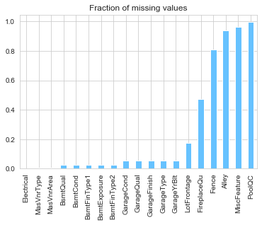
As listed above, certain features contain outliers. We can plot a bar plot of the proportion of missing values. This inspection will help target the specific features which require some additional work.

# count missing values per features
missing_fraction = train.isnull().sum() / train.shape[0]

# filter to keep only features with missing values
missing_fraction = missing_fraction[missing_fraction > 0]

# sort by highest ratio
missing_fraction = missing_fraction.sort_values()

# plot
missing_fraction.plot.bar(title='Fraction of missing values')

print("There are {} features with missing values.".format(missing_fraction.shape[0]))

There are 19 features with missing values.

We now inspect the distribution of our target feature. Indeed, most machine learning model perform well is the target feature is normally distributed. To check if it is the case, we can plot the distribution of the sale prices against standard distribution (Normal, Log…).

y = train['SalePrice']

mu, sigma = norm.fit(y)
sns.distplot(y, fit=norm)
plt.legend(['Normal distribution ($$\mu=$$ {:.2f} and $$\sigma=$$ {:.2f} )'.format(mu, sigma)], loc = 'best')
plt.ylabel('Frequency')
plt.title('Histogram of SalePrice');

fig = plt.figure()
res = probplot(y, plot=plt);

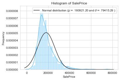
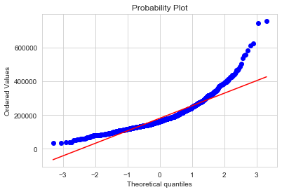
The above plots show that the sale price does cannot be approximated by a normal distribution. Indeed, the distribution plot and quantile-quantile plots are too different from the ones of a normal distribution.

plt.figure(1)
plt.title('Normal')
sns.distplot(y, kde=False, fit=stats.norm)

plt.figure(2)
plt.title('Log Normal')
sns.distplot(y, kde=False, fit=stats.lognorm)

plt.figure(3)
plt.title('Johnson SU')
sns.distplot(y, kde=False, fit=stats.johnsonsu)

plt.figure(4)
plt.title('Johnson SB')
sns.distplot(y, kde=False, fit=stats.johnsonsb);

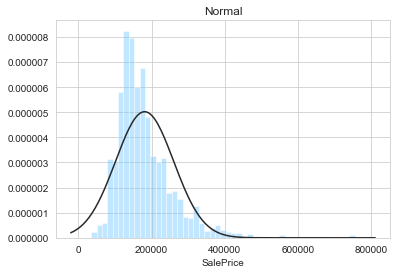
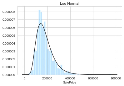
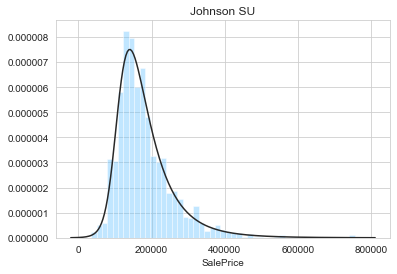
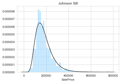
From the above figures, it appears that the sale prices are not normally distributed. Indeed, the log-normal, Johnson SU, and Johnson SB are the best fit. By visual inspection, the best fit is obtained with the Johnson SU distribution. We can now modify the target feature accordingly.

We can also test the numerical features to determine if they are approximately normally distributed.

numerical_features = [feature for feature in train.columns if train.dtypes[feature]!='object'] 
qualitive_features = [feature for feature in train.columns if train.dtypes[feature]=='object']

shapiro_test = lambda x: stats.shapiro(x.fillna(0))[1] > 0.05
shapiro_test_results = pd.DataFrame(train[numerical_features]).apply(shapiro_test)
print("{} feature distributions can be considered as drawn from a normal distribution.".format(shapiro_test_results.sum()))
print("Shapiro test significance level set to 0.05.")

0 feature distributions can be considered as drawn from a normal distribution.
Shapiro test significance level set to 0.05.

In addition to the target feature, none of the other numerical feature can be considered normally distributed.

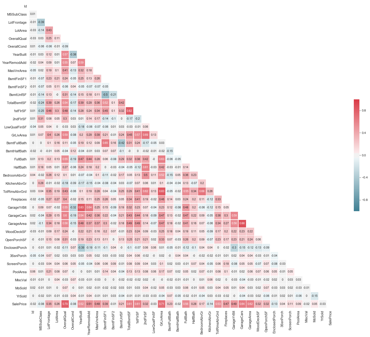
# Compute the correlation matrix
corr = train.corr()
corr = corr.round(decimals=2)

# Generate a mask for the upper triangle
mask = np.zeros_like(corr, dtype=np.bool)
mask[np.triu_indices_from(mask)] = True

# Set up the matplotlib figure
f, ax = plt.subplots(figsize=(22, 22))

# Generate a custom diverging colormap
cmap = sns.diverging_palette(220, 10, as_cmap=True)

# Draw the heatmap with the mask and correct aspect ratio
print("Correlation Map:")
sns.heatmap(corr, mask=mask, cmap=cmap, vmax=1.0,vmin=-1.0, center=0,annot=True,
            square=True, linewidths=.5,cbar_kws={"shrink": .3},annot_kws={"size":9},fmt='.2g',)
plt.tick_params(axis='both', which='major', labelsize=11);

Correlation Map:

2.3.1 Interior

The following variables are assigned to the “Interior” group.

Bsmt Qual (Ordinal): Evaluates the height of the basement
Bsmt Cond (Ordinal): Evaluates the general condition of the basement
Bsmt Exposure (Ordinal): Refers to walkout or garden level walls
BsmtFin Type 1 (Ordinal): Rating of basement finished area
BsmtFin SF 1 (Continuous): Type 1 finished square feet
BsmtFinType 2 (Ordinal): Rating of basement finished area (if multiple types)
BsmtFin SF 2 (Continuous): Type 2 finished square feet
Bsmt Unf SF (Continuous): Unfinished square feet of basement area
Total Bsmt SF (Continuous): Total square feet of basement area
1st Flr SF (Continuous): First Floor square feet
2nd Flr SF (Continuous) : Second floor square feet
Low Qual Fin SF (Continuous): Low quality finished square feet (all floors)
Bsmt Full Bath (Discrete): Basement full bathrooms
Bsmt Half Bath (Discrete): Basement half bathrooms
Full Bath (Discrete): Full bathrooms above grade
Half Bath (Discrete): Half baths above grade
Bedroom (Discrete): Bedrooms above grade (does NOT include basement bedrooms)
Kitchen (Discrete): Kitchens above grade
KitchenQual (Ordinal): Kitchen quality
TotRmsAbvGrd (Discrete): Total rooms above grade (does not include bathrooms)
Fireplaces (Discrete): Number of fireplaces
FireplaceQu (Ordinal): Fireplace quality
Gr Liv Area (Continuous): Above grade (ground) living area square feet

sns.set()
sns.set_style("whitegrid")
sns.set_palette(palette = mycols, n_colors = 4)

def plot_cat_feature_eda(featureName, order=None):
    fig, axarr = plt.subplots(1,4,figsize =(20, 8),sharey=True)
    
    # plot
    #plt.subplot(1,4,1)
    sns.boxplot(x=featureName, y='SalePrice',data=train,order=order,ax=axarr[0])
    axarr[0].set_xticklabels(axarr[0].get_xticklabels(), rotation=45)  
    
    #plt.subplot(1,4,2)
    plot = sns.violinplot(x=featureName, y='SalePrice',data=train, showmeans=False,
                          showmedians=False,showextrema=False,order=order,ax=axarr[1])
    axarr[1].set_ylabel("")
    axarr[1].set_xticklabels(axarr[1].get_xticklabels(), rotation=45)  
    
    #plt.subplot(1,4,3)
    plot = sns.swarmplot(x=featureName, y='SalePrice',data=train,order=order,ax=axarr[2])
    axarr[2].set_ylabel("")
    axarr[2].set_xticklabels(axarr[2].get_xticklabels(), rotation=45)  
    
    #plt.subplot(1,4,4)
    sns.barplot(x=featureName, y='SalePrice',data=train,
                order=order,ax=axarr[3])
    axarr[3].set_ylabel("")
    axarr[0].set_ylim(0,train['SalePrice'].max()*1.05)
    axarr[3].set_xticklabels(axarr[3].get_xticklabels(), rotation=45)  
    plt.suptitle(featureName);

feature = 'BsmtQual'
order = ['Fa', 'TA', 'Gd', 'Ex']
plot_cat_feature_eda(feature, order)

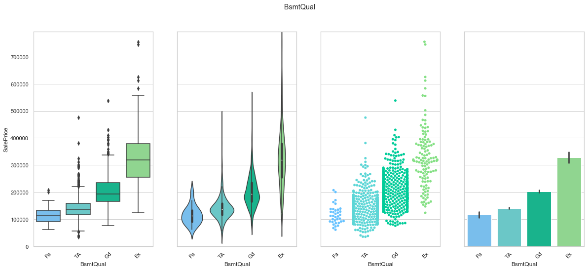
COMMENT: We found an order of the classes for BsmtQual that produces an increase in the sale price. We will use this to create a ordinal feature. Most of the data is contained within the “TA” and “Gd” groups.

feature = 'BsmtCond'
order = ['Po', 'Fa', 'TA', 'Gd']
plot_cat_feature_eda(feature, order)

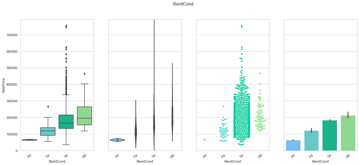
COMMENT: We found an order of the classes for BsmtCond that produces an increase in the sale price. We will use this to create a ordinal feature. Most of the data is contained within the “TA” group.

feature = 'BsmtExposure'
order = ['No', 'Mn', 'Av', 'Gd']
plot_cat_feature_eda(feature, order)

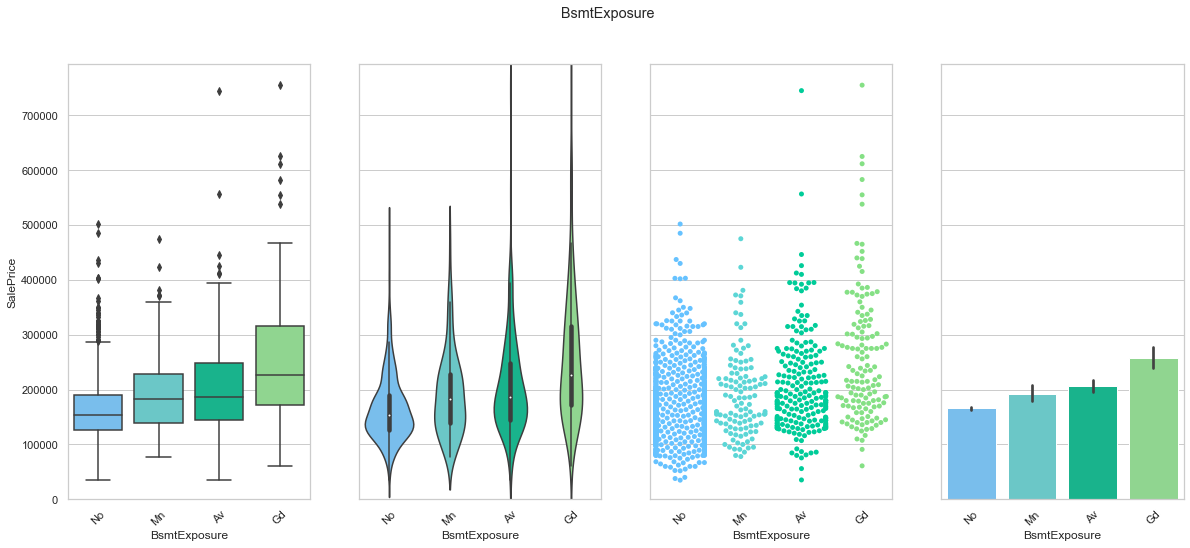
COMMENT: We found an order of the classes for BsmtExposure that produces an increase in the sale price. We will use this to create a ordinal feature. Most of the data is contained within the “No” group.

feature = 'BsmtFinType1'
order = ["Unf", "LwQ", "Rec", "BLQ", "ALQ", "GLQ"]
plot_cat_feature_eda(feature, order)

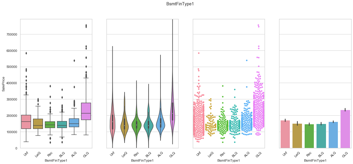
COMMENT: From the above data, it seems that a house with an unfinished basement has more value than any other type of basement except for the ones with a good quality. Since the order of the categories is not obvious, we will create dummy features.

def plot_num_feature_eda(featureName):
    plt.subplots(figsize =(30, 20))
    grid = plt.GridSpec(2, 3, wspace=0.1, hspace=0.15)
    
    # plot
    plt.subplot(grid[0, 0])
    g = sns.regplot(x=train[feature], y=train['SalePrice'], fit_reg=False)
    g.axes.set_xlim(0,)
    g.axes.set_ylim(0,)
    
    # plot
    plt.subplot(grid[0, 1:])
    sns.boxplot(x='Neighborhood', y=feature, data=train, palette = mycols)
    
    # plot
    plt.subplot(grid[1, 0]);
    sns.boxplot(x='BldgType', y=feature, data=train, palette = mycols)
    
    # plot
    plt.subplot(grid[1, 1]);
    sns.boxplot(x='HouseStyle', y=feature, data=train, palette = mycols)
    
    # plot
    plt.subplot(grid[1, 2]);
    sns.boxplot(x='LotShape', y=feature, data=train, palette = mycols)
    print(featureName);

feature = 'BsmtFinSF1'
plot_num_feature_eda(feature)

BsmtFinSF1

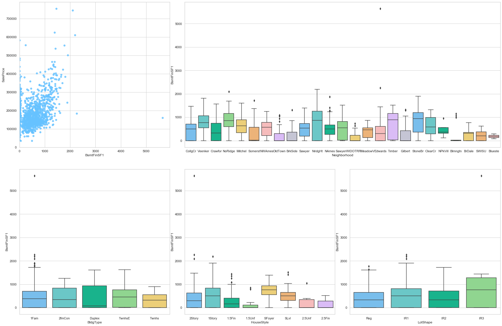
COMMENT:

From the first plot, we observe a positive correlation between the sale prince and the Type 1 finished sft.
From the box plot, we notice that the distribution of the sale price as function of the Type 1 finished sft is strongly linked to the neighborhood.
The last three boxplots also show a strong dependence to the architecture (Building type, house style, and lot shape).

feature = 'BsmtFinType2'
order = ['Unf', 'BLQ', 'ALQ', 'Rec', 'LwQ', 'GLQ']
plot_cat_feature_eda(feature, order)

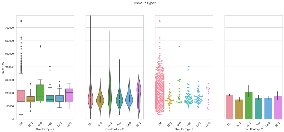
COMMENT:

Most of the data is contained in the “Unfinished” group.
The distribution of the data does not indicate that the sale price increases with the quality of the finish for the second basement.

feature = 'BsmtFinSF2'
plot_num_feature_eda(feature)

BsmtFinSF2

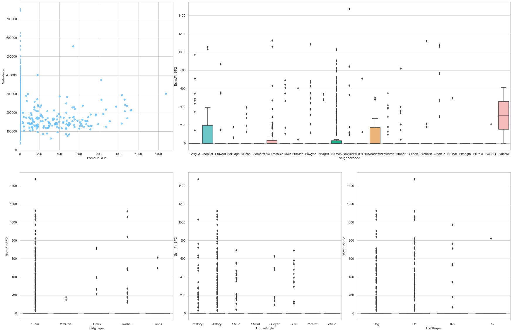
COMMENT:

A large portion of the data is associated to the value 0.
There is no clear correlation between the sale price and this feature.

feature = 'BsmtUnfSF'
plot_num_feature_eda(feature)

BsmtUnfSF

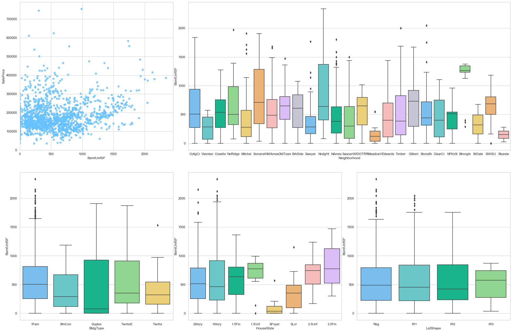
COMMENT

This feature is positively correlated to the sale price. A fraction of the data is assigned a 0 value.
The area of unfinished basement varies greatly from one neighborhood to the other.
The same conclusion can be made when looking at the type of house.

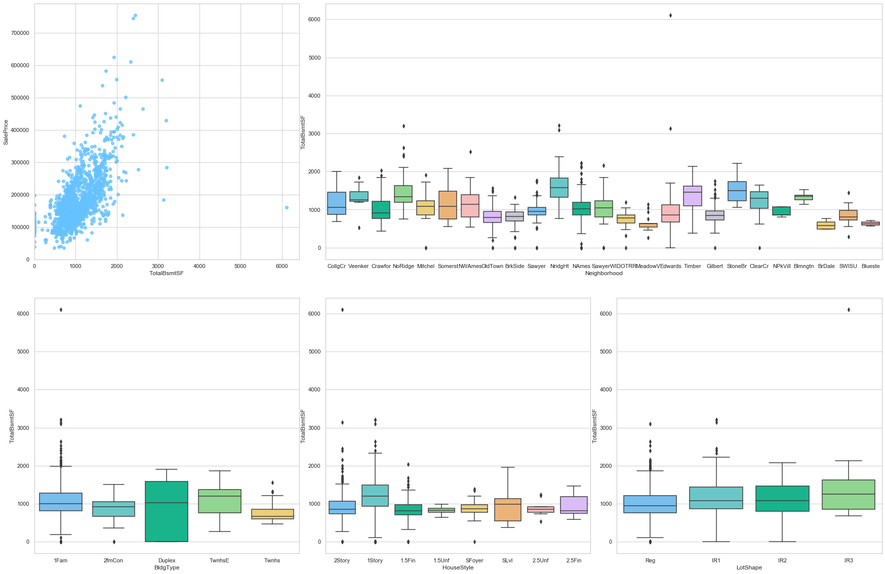
feature = 'TotalBsmtSF'
plot_num_feature_eda(feature)

TotalBsmtSF

COMMENT

This feature is strongly positively correlated to the sale price. A small fraction of the data is assigned a 0 value.
The area of unfinished basement varies greatly from one neighborhood to the other.
However, the type of the house does not have a large impact on this feature.

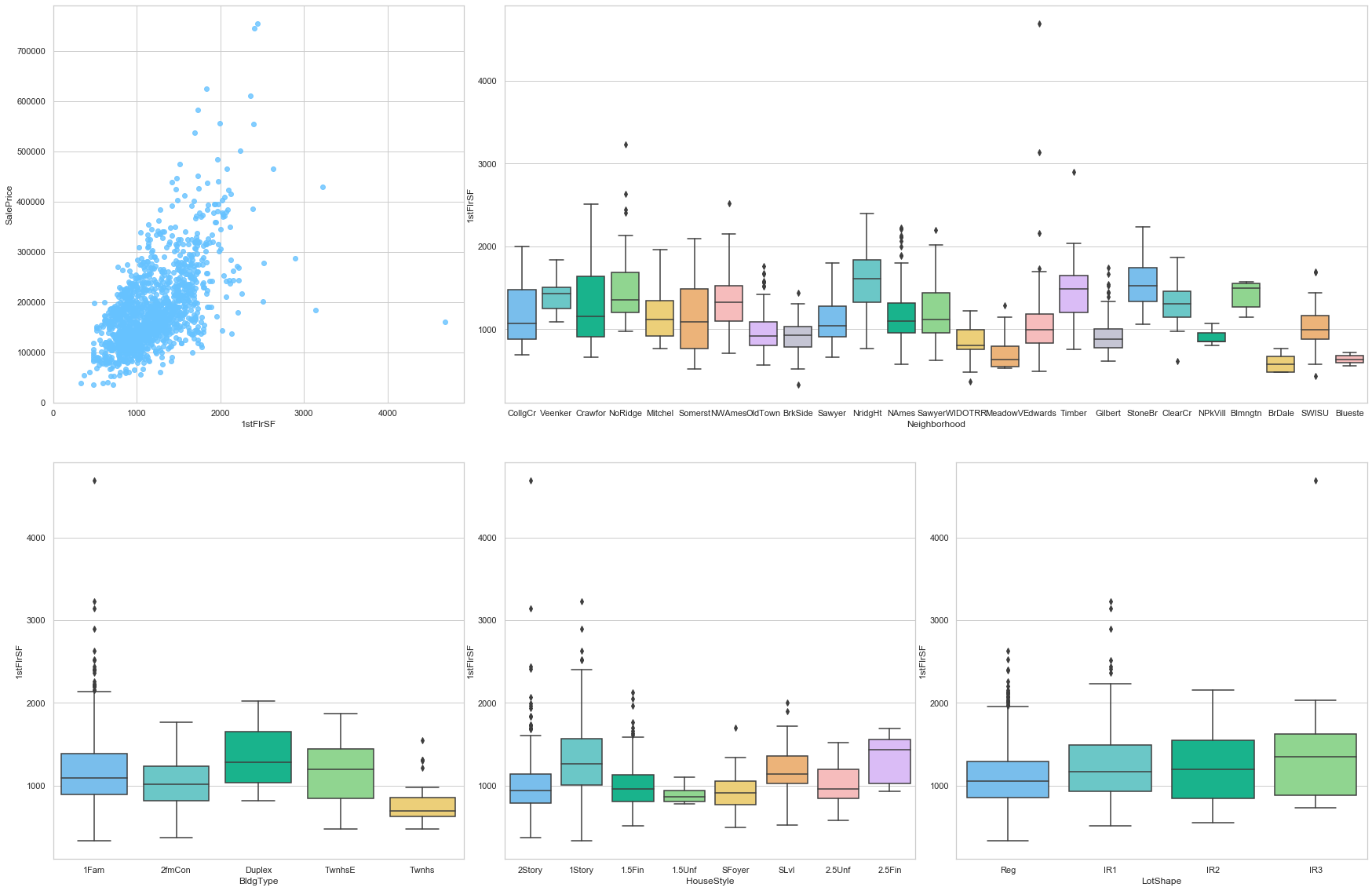
feature = '1stFlrSF'
plot_num_feature_eda(feature)

1stFlrSF

COMMENT

This feature is strongly positively correlated to the sale price.
The surface of the first floor varies greatly from one neighborhood to the other.
However, the type of the house does not have a large impact on this feature.

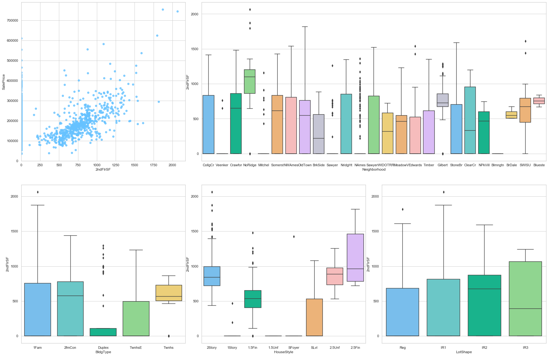
feature = '2ndFlrSF'
plot_num_feature_eda(feature)

2ndFlrSF

COMMENT

This feature is strongly positively correlated to the sale price. Moreover, a large number of data points are assigned to the value 0. This can be explained because a large number of individual houses are only built with one floor.
The surface of the second floor varies greatly from one neighborhood to the other.
However, the type of the house does not have a large impact on this feature.

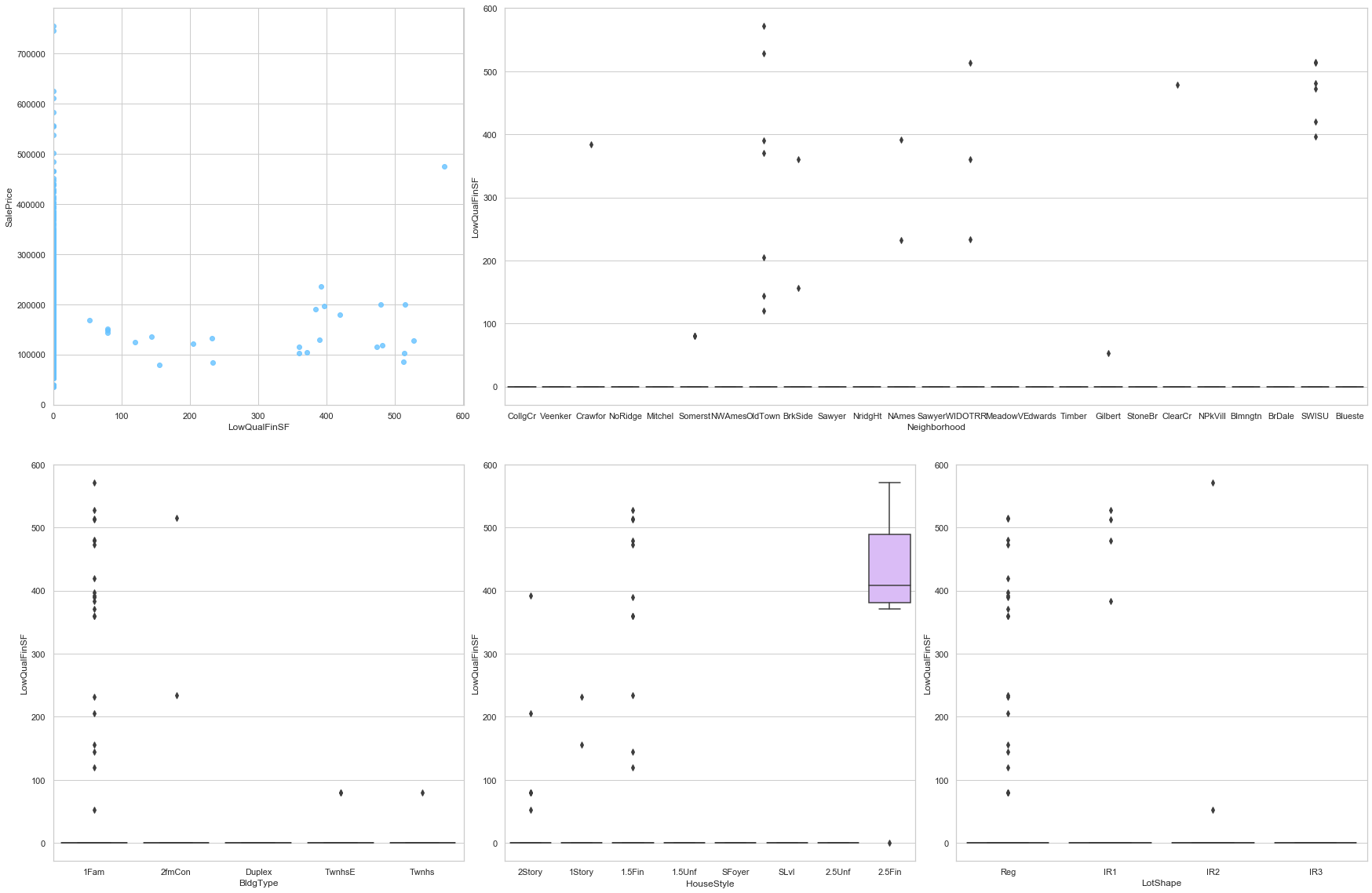
feature = 'LowQualFinSF'
plot_num_feature_eda(feature)

LowQualFinSF

COMMENT

Most of the data is assigned the value 0.

feature = 'BedroomAbvGr'
plot_cat_feature_eda(feature)

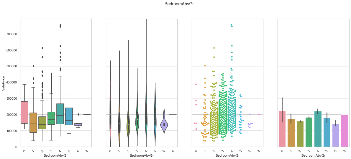
COMMENT

Most houses have between two and four bedrooms above grade level.

feature = 'KitchenAbvGr'
plot_cat_feature_eda(feature)

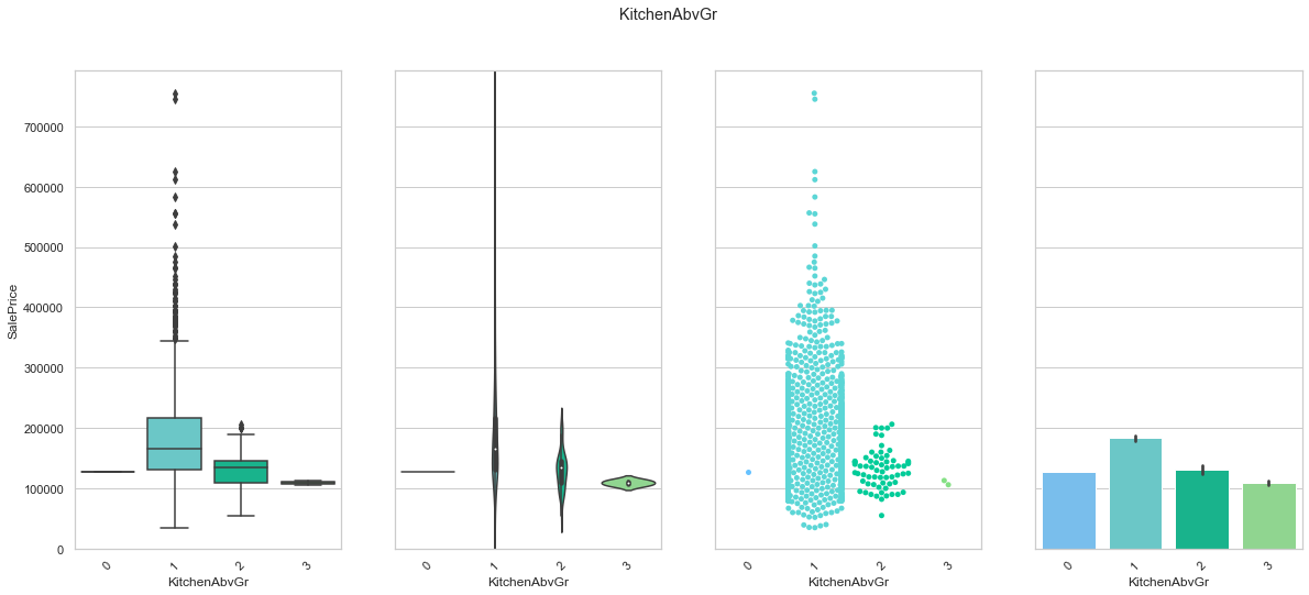
COMMENT

Most houses have one single kitchen.

feature = 'KitchenQual'
order = ['Fa', 'TA', 'Gd', 'Ex']
plot_cat_feature_eda(feature, order)

COMMENT: We found an order of the classes for KitchenQual that produces an increase in the sale price. We will use this to create a ordinal feature.

feature = 'TotRmsAbvGrd'
plot_cat_feature_eda(feature)

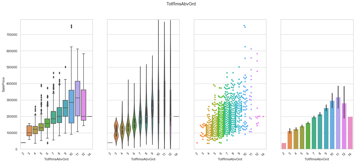
COMMENT

There seems to be a positive correlation between the number of rooms and the sale prince.
The extreme classes (2, 12, and 14) do not have enough data for to be reliable.

feature = 'Fireplaces'
plot_cat_feature_eda(feature)

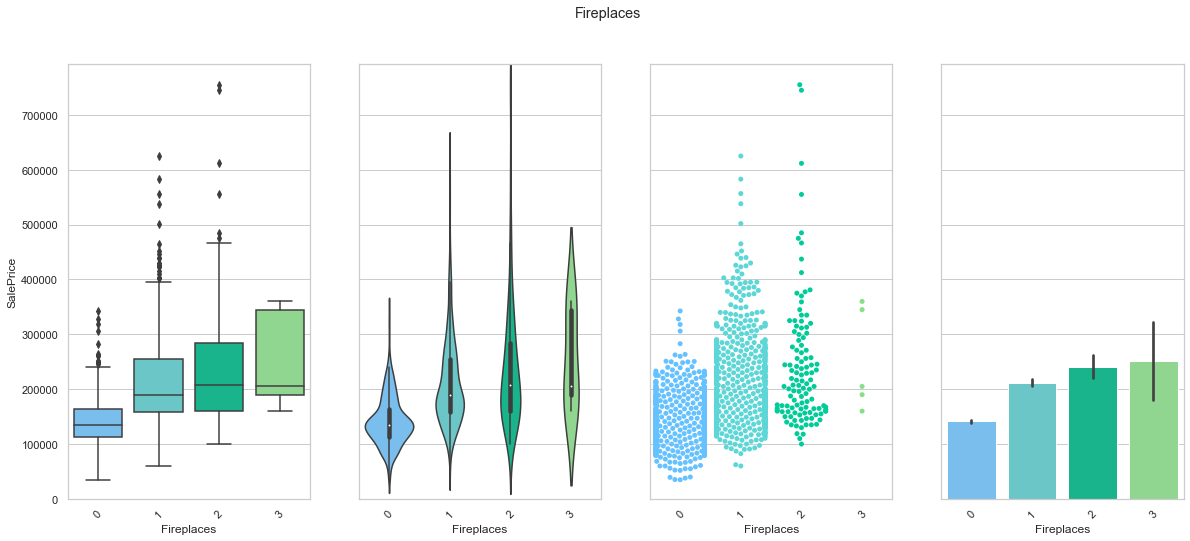
COMMENT

There seems to be a positive correlation between the number of fireplaces and the sale prince.
The extreme class (3) do not have enough data for to be reliable.

train['FireplaceQu'].unique()

array([nan, 'TA', 'Gd', 'Fa', 'Ex', 'Po'], dtype=object)

feature = 'FireplaceQu'
order = ["Po", "Fa", "TA", "Gd", "Ex"]
plot_cat_feature_eda(feature, order)

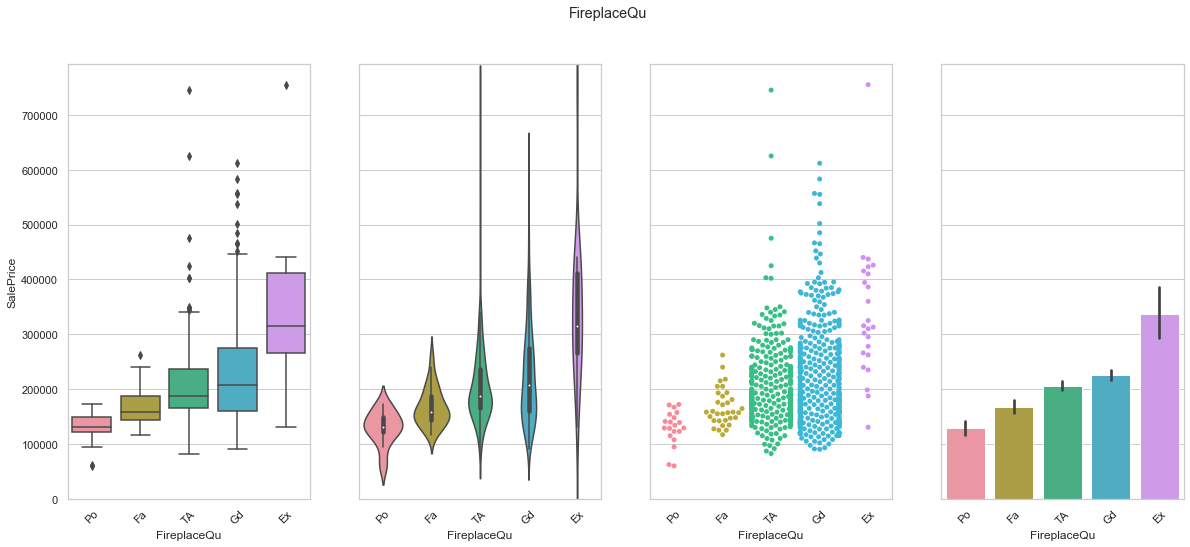
COMMENT: We found an order of the classes for FireplaceQu that produces an increase in the sale price. We will use this to create a ordinal feature.

GrLivArea

feature = 'GrLivArea'
plot_num_feature_eda(feature)

GrLivArea

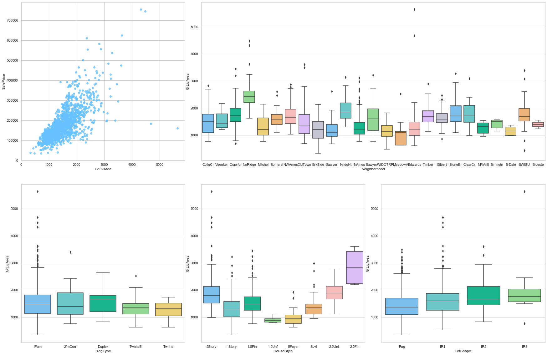
COMMENT

This feature is strongly positively correlated to the sale price. Moreover, a large number of data points are assigned to the value 0. This can be explained because a large number of individual houses are only built with one floor.
This feature varies greatly from one neighborhood to the other.
However, the type of the house does not have a large impact on this feature.

2.3.2 Exterior

The following variables are assigned to the “Exterior” group.

MS SubClass (Nominal): Identifies the type of dwelling involved in the sale.
Bldg Type (Nominal): Type of dwelling
House Style (Nominal): Style of dwelling
Overall Qual (Ordinal): Rates the overall material and finish of the house
Overall Cond (Ordinal): Rates the overall condition of the house
Year Built (Discrete): Original construction date
Year Remod/Add (Discrete): Remodel date (same as construction date if no remodeling or additions)
Foundation (Nominal): Type of foundation
Functional (Ordinal): Home functionality (Assume typical unless deductions are warranted)
Roof Style (Nominal): Type of roof
Roof Matl (Nominal): Roof material
Exterior 1 (Nominal): Exterior covering on house
Exterior 2 (Nominal): Exterior covering on house (if more than one material)
Mas Vnr Type (Nominal): Masonry veneer type
Mas Vnr Area (Continuous): Masonry veneer area in square feet
Exter Qual (Ordinal): Evaluates the quality of the material on the exterior
Exter Cond (Ordinal): Evaluates the present condition of the material on the exterior
Garage Type (Nominal): Garage location
Garage Yr Blt (Discrete): Year garage was built
Garage Finish (Ordinal) : Interior finish of the garage
Garage Cars (Discrete): Size of garage in car capacity
Garage Area (Continuous): Size of garage in square feet
Garage Qual (Ordinal): Garage quality
Garage Cond (Ordinal): Garage condition
Wood Deck SF (Continuous): Wood deck area in square feet
Open Porch SF (Continuous): Open porch area in square feet
Enclosed Porch (Continuous): Enclosed porch area in square feet
3-Ssn Porch (Continuous): Three season porch area in square feet
Screen Porch (Continuous): Screen porch area in square feet
Pool Area (Continuous): Pool area in square feet
Pool QC (Ordinal): Pool quality
Fence (Ordinal): Fence quality

feature = 'MSSubClass'
plot_cat_feature_eda(feature)

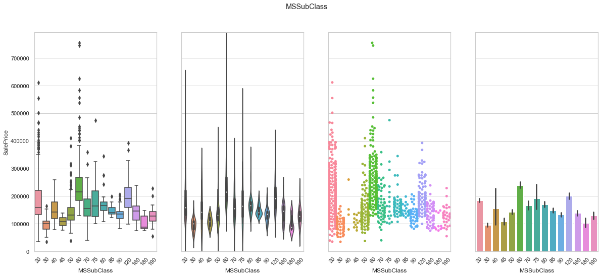
COMMENT

Although this feature contains numerical value, it is meant to describe building style. We therefore turn the data into strings.

feature = 'BldgType'
plot_cat_feature_eda(feature)

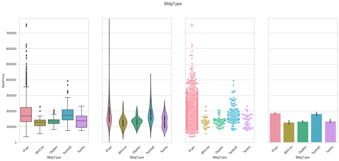
COMMENT

The feature is transformed using dummies.

feature = 'HouseStyle'
plot_cat_feature_eda(feature)

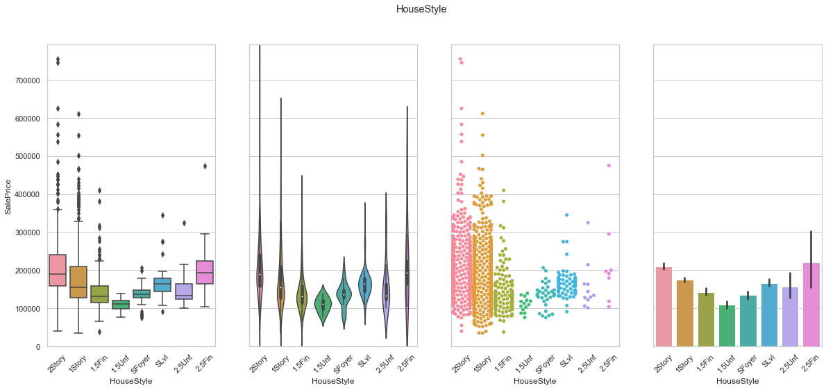
COMMENT

The first two categories present a large number of extremely high values.
This feature is turned into a set of dummy variables.

feature = 'OverallQual'
plot_cat_feature_eda(feature)

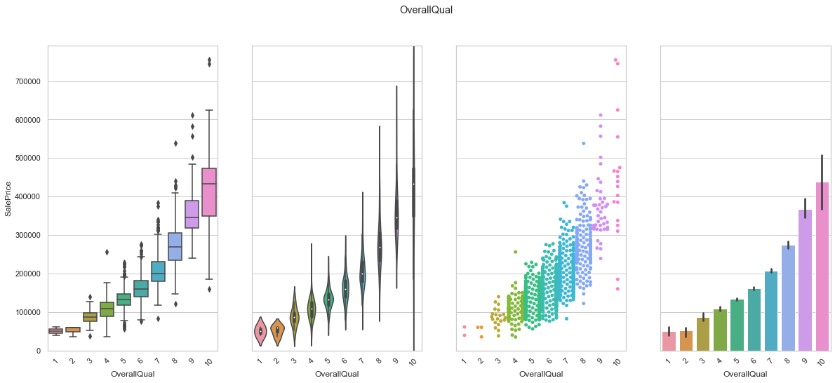
COMMENT

As expected, the overall quality is strongly positively correlated to the sale price.

feature = 'OverallCond'
plot_cat_feature_eda(feature)

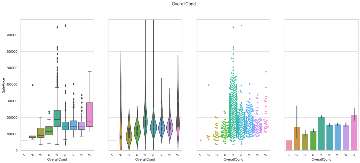
COMMENT

As expected, the overall condition is correlated to the sale price. However, the class corresponding to a value of 5 has a higher meadian sale price than the class corresponding to the value 9.

import matplotlib.ticker as ticker

def plot_date_feature(featureName, stepsize=5):
    fig, axarr = plt.subplots(3,1,figsize =(20, 20))
    
    # plot
    #plt.subplot(1,4,1)
    sns.boxplot(x=feature, y='SalePrice',data=train,ax=axarr[0])
    axarr[0].set_xticklabels(axarr[0].get_xticklabels(), rotation=45)  
    
    # plot
    #plt.subplot(1,4,3)
    plot = sns.swarmplot(x=feature, y='SalePrice',data=train,ax=axarr[1])
    axarr[1].set_ylabel("")
    axarr[1].set_xticklabels(axarr[1].get_xticklabels(), rotation=45)
    
    # purpose
    #plt.subplot(1,4,4)
    sns.barplot(x=feature, y='SalePrice',data=train,ax=axarr[2])
    axarr[2].set_ylabel("")
    axarr[0].set_ylim(0,train['SalePrice'].max()*1.05)
    axarr[2].set_xticklabels(axarr[2].get_xticklabels(), rotation=45)
    
    for label in axarr[0].get_xticklabels():
        label.set_visible(float(label._text) % stepsize==0)
    for label in axarr[1].get_xticklabels():
        label.set_visible(float(label._text) % stepsize==0)
    for label in axarr[2].get_xticklabels():
        label.set_visible(float(label._text) % stepsize==0)
    
    plt.suptitle(featureName)
    plt.tight_layout();

feature = 'YearRemodAdd'
plot_date_feature(feature)

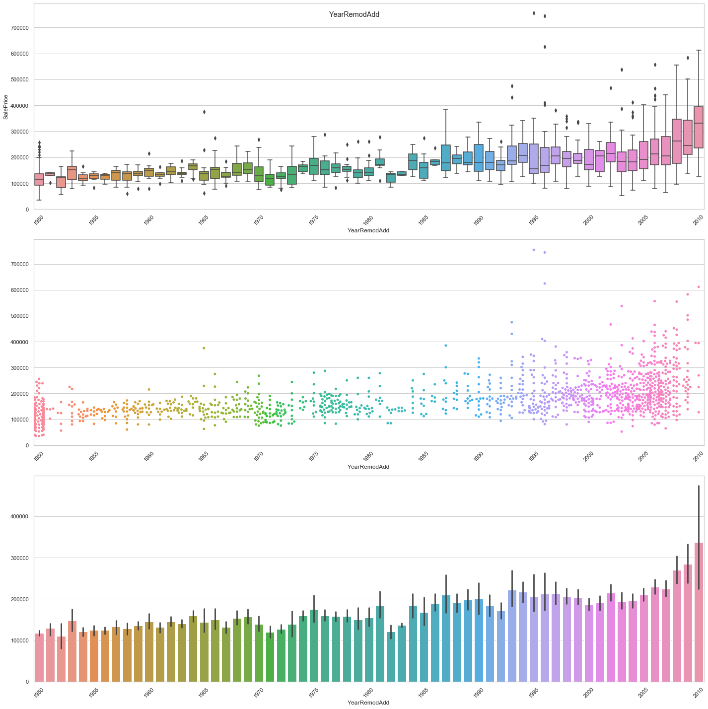
COMMENT

The newer the remodeling the higher the sale price.

feature = 'YearBuilt'
plot_date_feature(feature, stepsize=10)

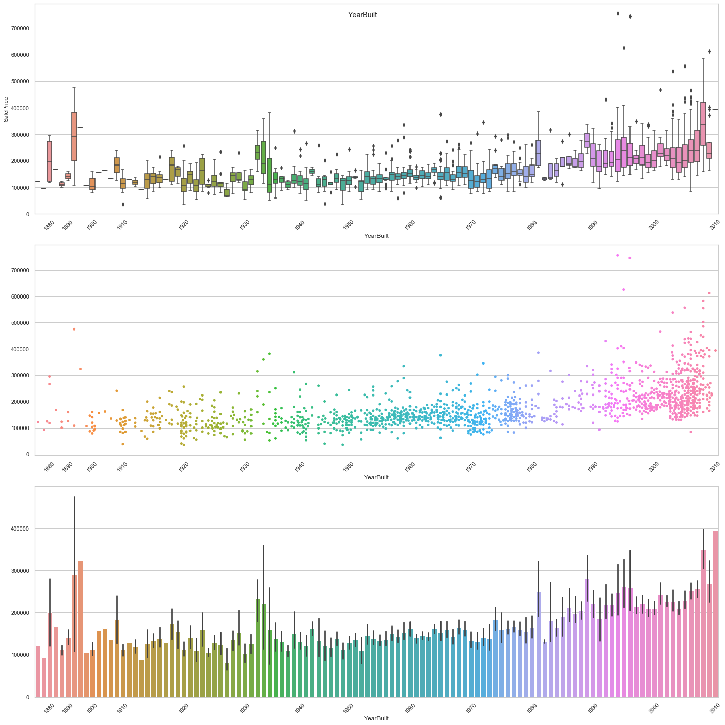
COMMENT

The general trend seems to depict a higher sale price for newer constructions.

feature = 'Foundation'
plot_cat_feature_eda(feature)

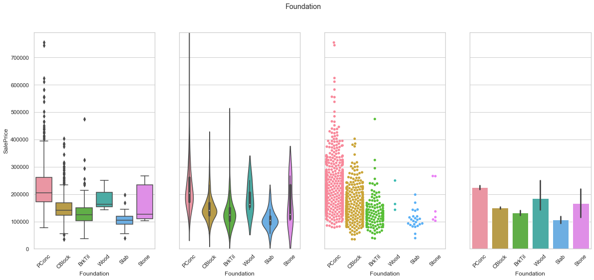
COMMENT

The data is mostly gathered into the first three classes.

feature = 'Functional'
plot_cat_feature_eda(feature)

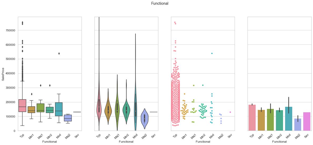
COMMENT

Most of the data is stored under the “Typ” class.
From the information about the dataset, we can identify an order with which the classes can be organized. The “Typ” class corresponds to the highest rank within this ordinal feature.

feature = 'RoofStyle'
plot_cat_feature_eda(feature)

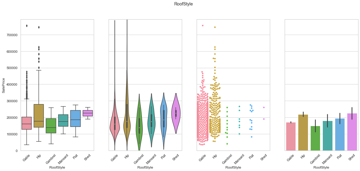
COMMENT

Most of the data is stored under the “Gable” and “Hip” classes.
We create dummy variables to store the data.

feature = 'RoofMatl'
plot_cat_feature_eda(feature)

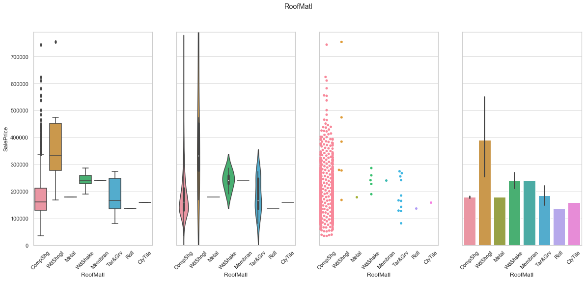
COMMENT

Almost the entire dataset is stored under “CompShg” class.

Exterior1st and Exterior2nd After inspection, it appears that most of the houses have the same class for the exterior features. We will use this to minimize the redundancy of the stored information.

feature = 'Exterior1st'
fig, axarr = plt.subplots(3,1,figsize =(20, 15),sharey=True)

# plot
sns.boxplot(x=feature, y='SalePrice',data=train,ax=axarr[0])

# plot
plot = sns.swarmplot(x=feature, y='SalePrice',data=train,ax=axarr[1])
axarr[1].set_ylabel("")

# purpose
sns.barplot(x=feature, y='SalePrice',data=train,ax=axarr[2])
axarr[2].set_ylabel("")
axarr[0].set_ylim(0,train['SalePrice'].max()*1.05);

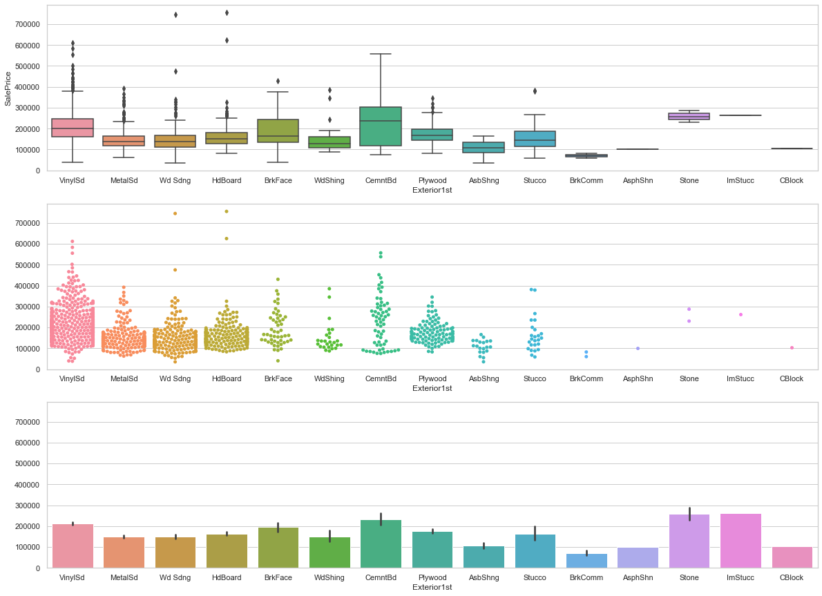
feature = 'Exterior2nd'
fig, axarr = plt.subplots(3,1,figsize =(20, 15),sharey=True)

# plot
sns.boxplot(x=feature, y='SalePrice',data=train,ax=axarr[0])

# plot
plot = sns.swarmplot(x=feature, y='SalePrice',data=train,ax=axarr[1])
axarr[1].set_ylabel("")

# purpose
sns.barplot(x=feature, y='SalePrice',data=train,ax=axarr[2])
axarr[2].set_ylabel("")
axarr[0].set_ylim(0,train['SalePrice'].max()*1.05);

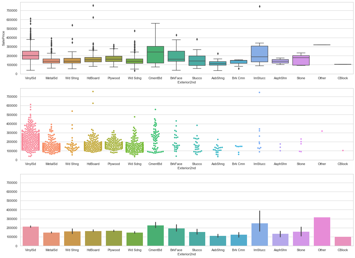
COMMMENT

Most records have the save value for both exterior features.

feature = 'MasVnrType'
plot_cat_feature_eda(feature)

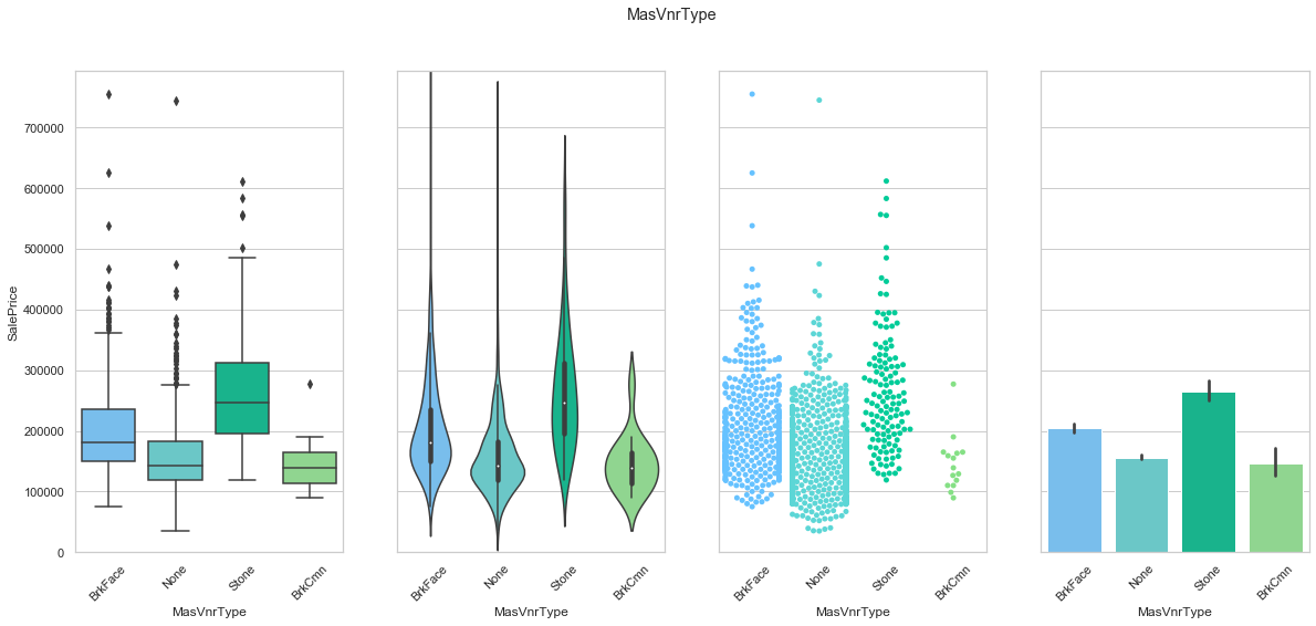
COMMENT

Each class leads to a different average sale price.
Most of the data is stored in the first three classes.

train['MasVnrArea'].isnull().count()

feature = 'MasVnrArea'
plot_num_feature_eda(feature)

MasVnrArea

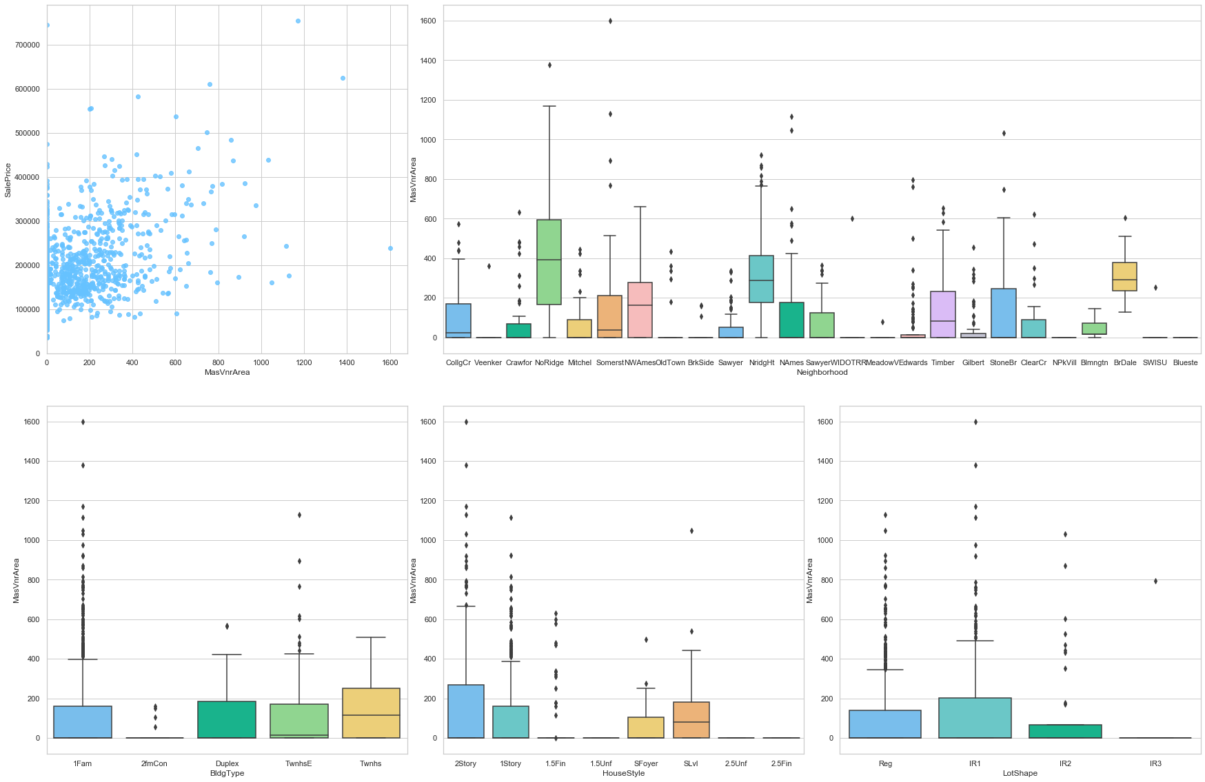
COMMENT

There is no clear correlation between this feature and the sale price.
Most of the data is assigned a value of 0.

feature = 'ExterQual'
order = ['Fa', 'TA', 'Gd', 'Ex']
plot_cat_feature_eda(feature, order)

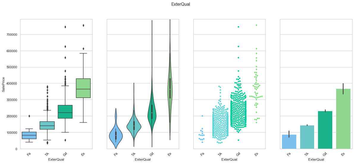
COMMENT

This is an ordinal feature. The classes are arrange to create an increase in sale price from one feature to another.
Most of the data is stored in the two central classes.

feature = 'ExterCond'
order = ['Po','Fa','TA','Gd', 'Ex']
plot_cat_feature_eda(feature, order)

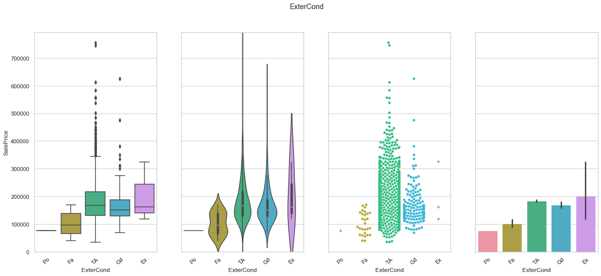
COMMENT

This is an ordinal feature but the sale price does not reflect the feature order.
Most of the data is stored in the two central classes.

feature = 'GarageType'
plot_cat_feature_eda(feature)

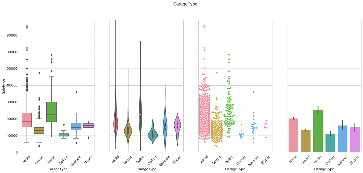
COMMENT

There is no real order within this categorical feature.

feature = 'GarageYrBlt'
plot_date_feature(feature)

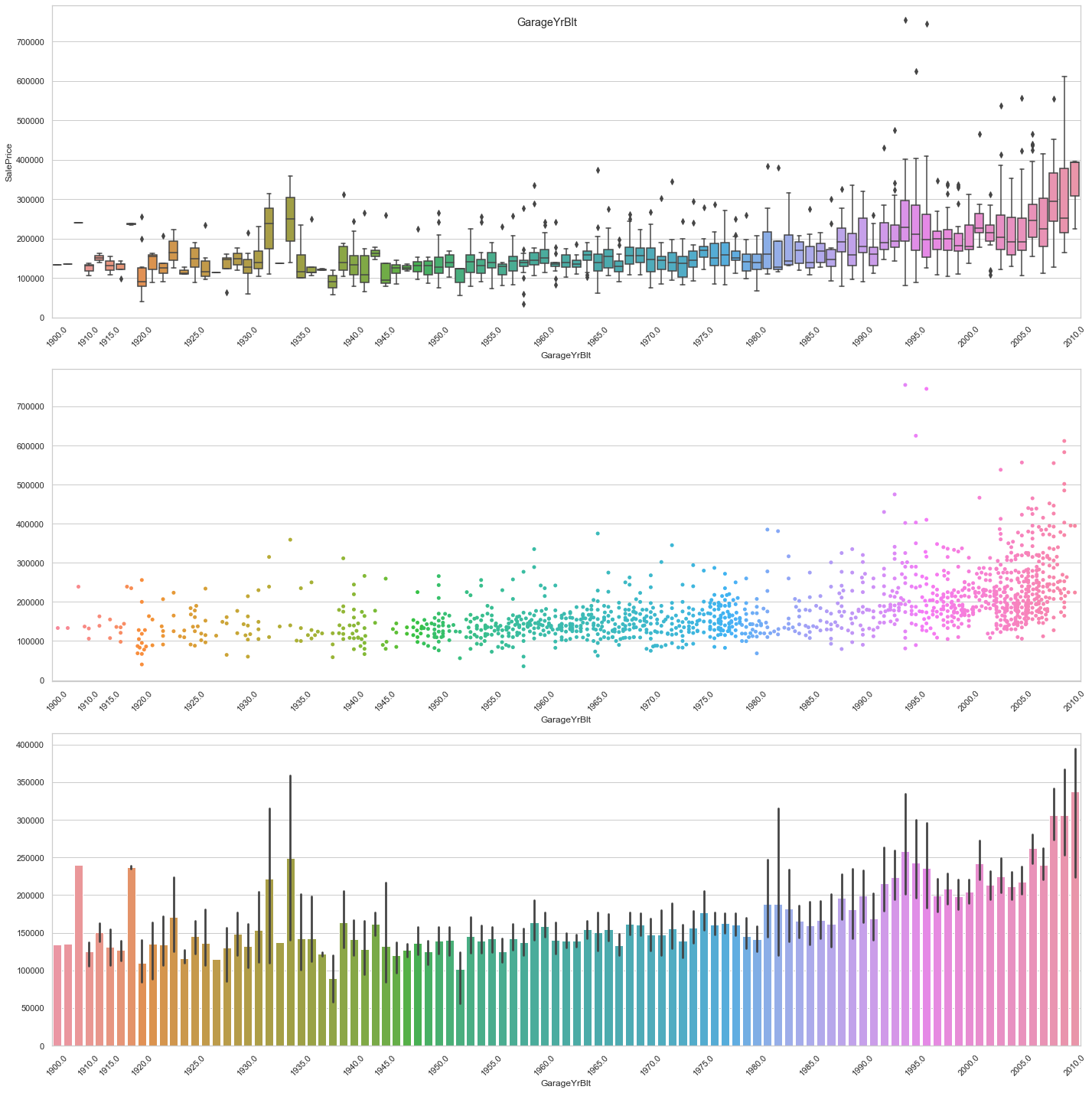
COMMENT

For recent constructions, it seems that there is an upward trend. For older constructions, the average sale price seems to be fairly constant.

feature = 'GarageFinish'
plot_cat_feature_eda(feature)

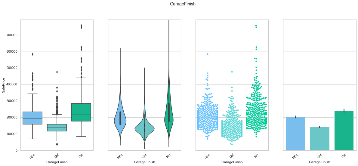
COMMENT

The data is evenly distributed amongst the three classes.

feature = 'GarageCars'
plot_cat_feature_eda(feature)

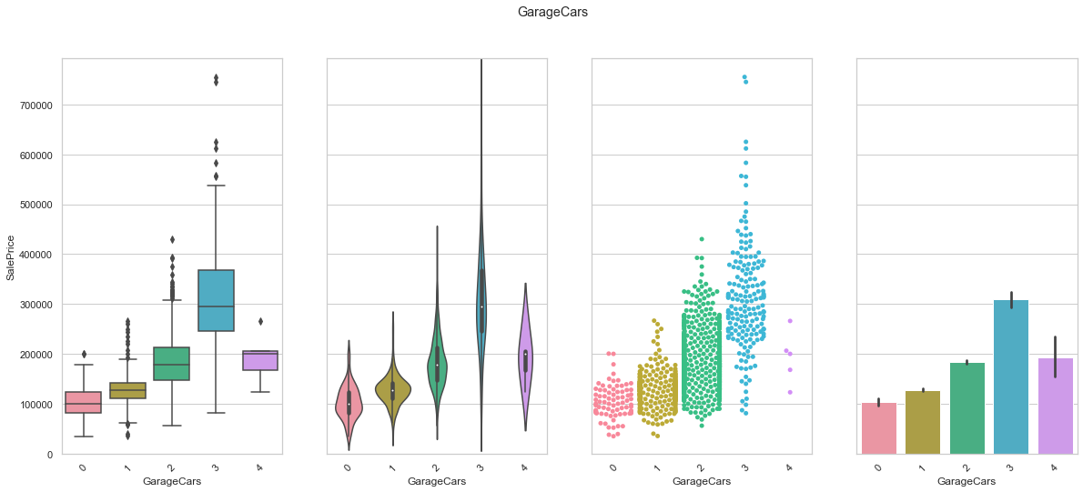
COMMENT

There is a clear increase in sale price from class 0 to class 3. However, class 4 does not follow this trend. This can be explained by the low number of records with 4 car spaces.

feature = 'GarageArea'
plot_num_feature_eda(feature)

GarageArea

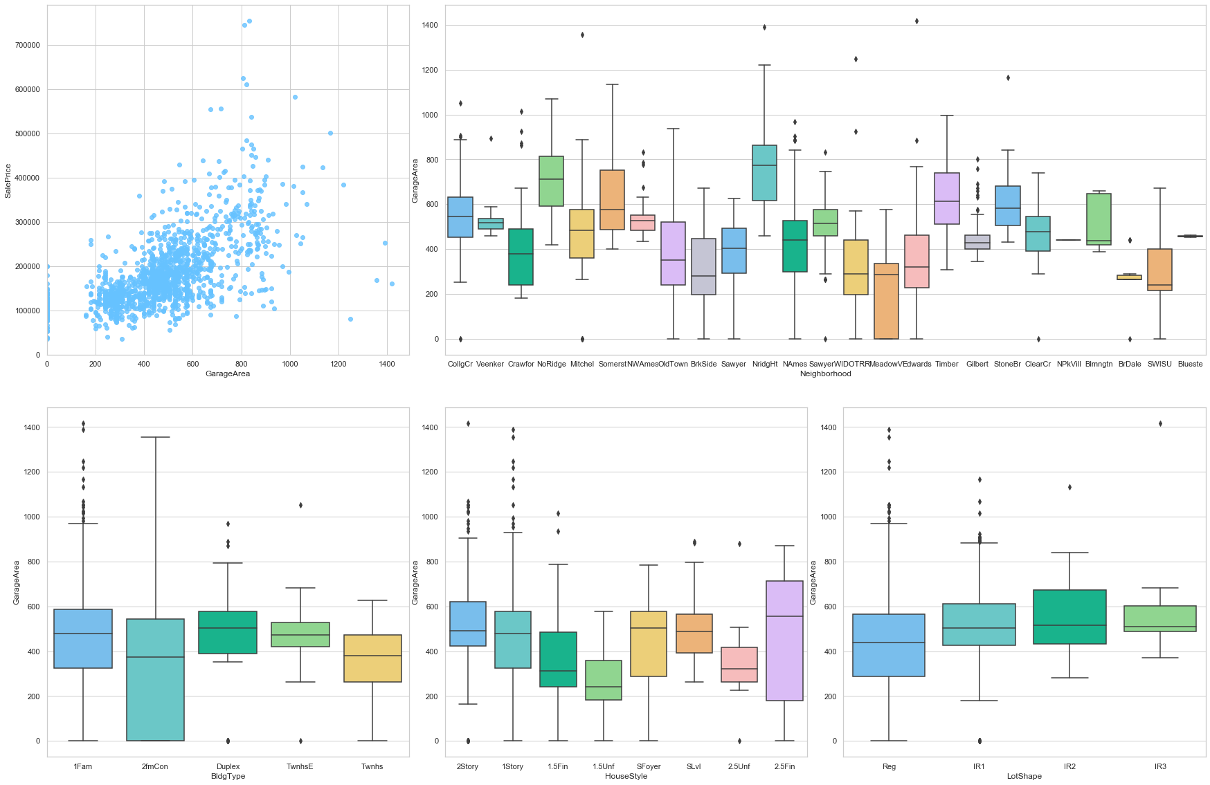
COMMENT

The sale price is strongly correlated to this feature (positive correlation).
There is a high variation of this feature when looking at the neighborhoods.

feature = 'GarageQual'
order=["Po", "Fa", "TA", "Gd", "Ex"]
plot_cat_feature_eda(feature, order)

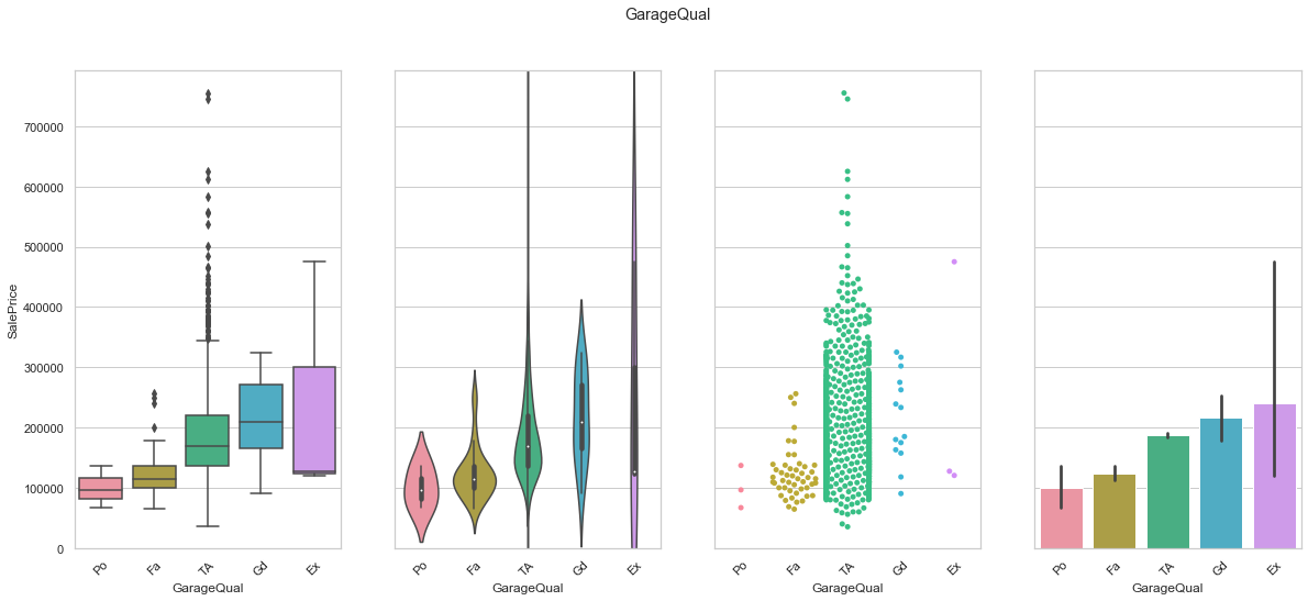
COMMENT

We found a sequence that leads to an increase in sale price. Only the Ex feature does not really match the ranking but the small number of Ex records is the reason for such a behavior.

feature = 'GarageCond'
order=["Po", "Fa", "TA", "Gd", "Ex"]
plot_cat_feature_eda(feature, order)

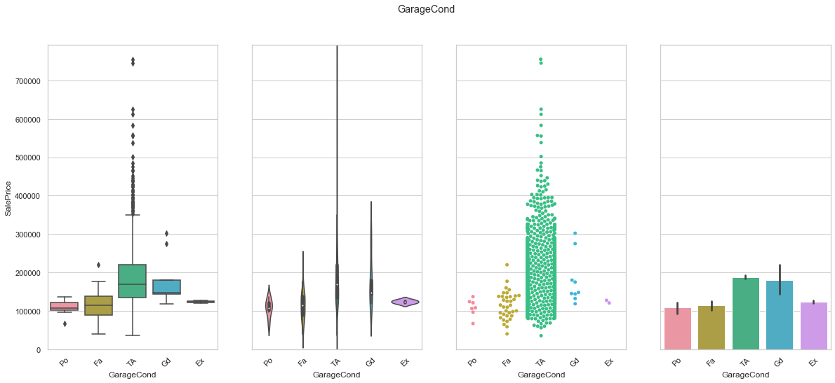
COMMENT

We found a sequence that leads to an increase in sale price. Only the Ex feature does not really match the ranking but the small number of Ex records is the reason for such a behavior.

feature = 'WoodDeckSF'
plot_num_feature_eda(feature)

WoodDeckSF

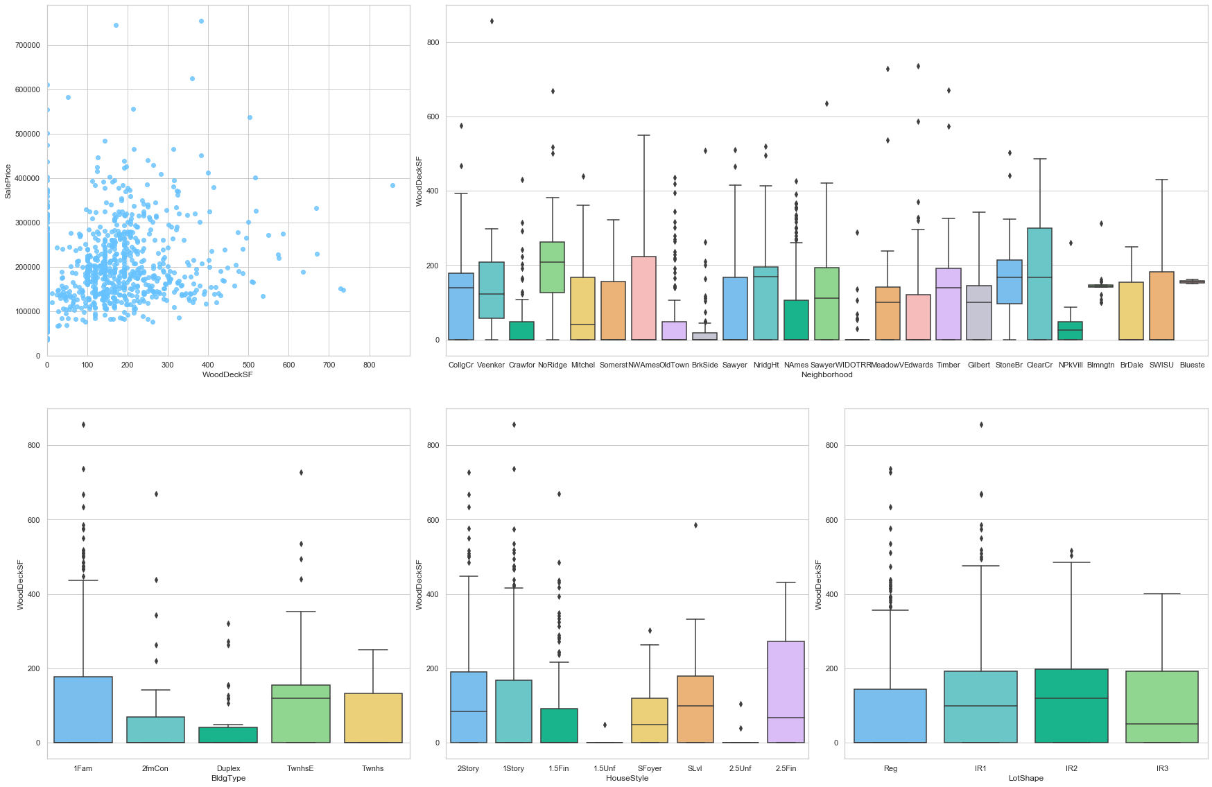
COMMENT

There is a good positive correlation between the sale price and this feature..
The neighborhood and location feature have a great impact on this feature.
A large number of data points are assigned the value 0.

feature = 'PoolArea'
plot_num_feature_eda(feature)

PoolArea

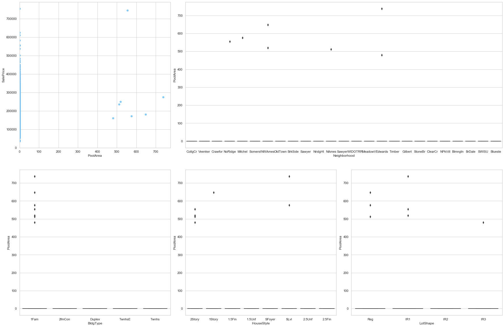
COMMENT

Most of the data is stored as 0. This feature may be dropped.

feature = 'Fence'
order=['MnWw', 'GdWo', 'MnPrv', 'GdPrv']
plot_cat_feature_eda(feature, order)

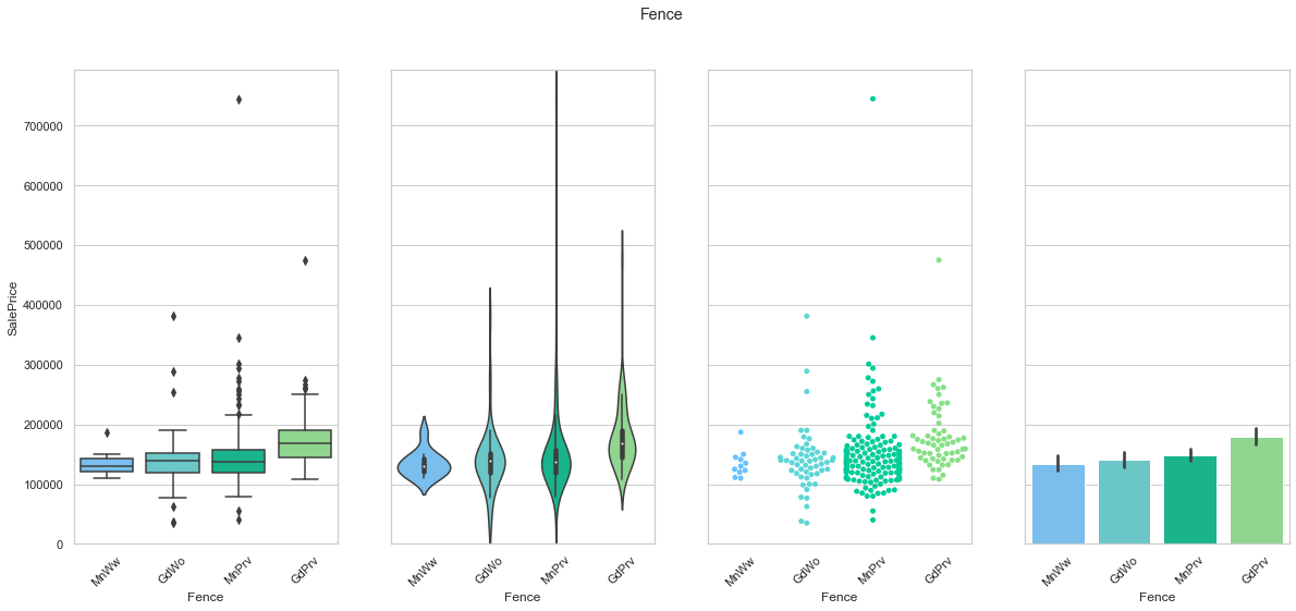
COMMENT

The data is mostly stored in a single class.
It is possibly to arrange the classes to create an ordinal sequence.

2.3.3. Miscellaneous

The following variables are assigned to the “Miscellaneous” group.

Order (Discrete): Observation number
PID (Nominal): Parcel identification number - can be used with city web site for parcel review.
MS Zoning (Nominal): Identifies the general zoning classification of the sale.
Lot Frontage (Continuous): Linear feet of street connected to property
Lot Area (Continuous): Lot size in square feet
Street (Nominal): Type of road access to property
Alley (Nominal): Type of alley access to property
Lot Shape (Ordinal): General shape of property
Land Contour (Nominal): Flatness of the property
Utilities (Ordinal): Type of utilities available
Lot Config (Nominal): Lot configuration
Land Slope (Ordinal): Slope of property
Neighborhood (Nominal): Physical locations within Ames city limits (map available)
Condition 1 (Nominal): Proximity to various conditions
Condition 2 (Nominal): Proximity to various conditions (if more than one is present)
Heating (Nominal): Type of heating
HeatingQC (Ordinal): Heating quality and condition
Central Air (Nominal): Central air conditioning
Electrical (Ordinal): Electrical system
Paved Drive (Ordinal): Paved driveway
Misc Feature (Nominal): Miscellaneous feature not covered in other categories
Misc Val (Continuous): $$Value of miscellaneous feature
Mo Sold (Discrete): Month Sold (MM)
Yr Sold (Discrete): Year Sold (YYYY)
Sale Type (Nominal): Type of sale
Sale Condition (Nominal): Condition of sale

feature = 'MSZoning'
plot_cat_feature_eda(feature)

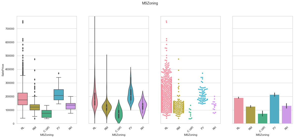
COMMENT

The data is mostly contained is a single class.

feature = 'Neighborhood'
order=None
fig, axarr = plt.subplots(3,1,figsize =(20, 15),sharey=True)

# plot
sns.boxplot(x=feature, y='SalePrice',data=train,ax=axarr[0],order=order)

# plot
plot = sns.swarmplot(x=feature, y='SalePrice',data=train,ax=axarr[1],order=order)
axarr[1].set_ylabel("")

# purpose
sns.barplot(x=feature, y='SalePrice',data=train,ax=axarr[2],order=order)
axarr[2].set_ylabel("")
axarr[0].set_ylim(0,train['SalePrice'].max()*1.05);

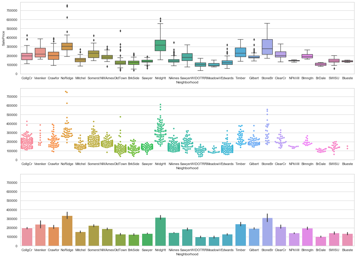
COMMENT

The location is obviously a key feature when predicting the price of an estate.

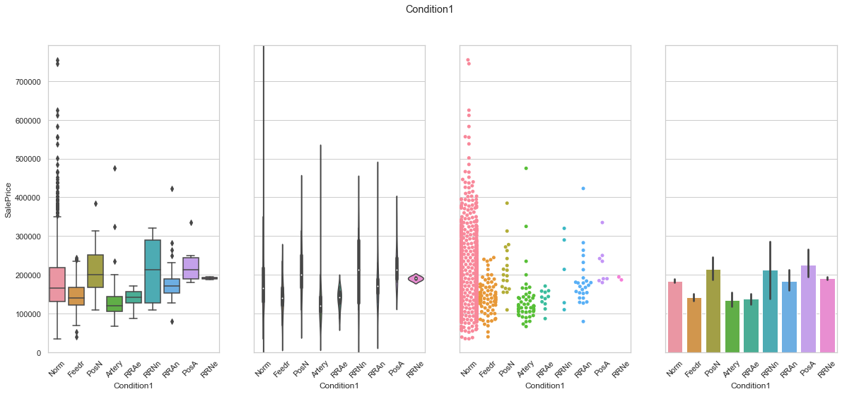
feature = 'Condition1'
plot_cat_feature_eda(feature)

feature = 'Condition2'
plot_cat_feature_eda(feature)

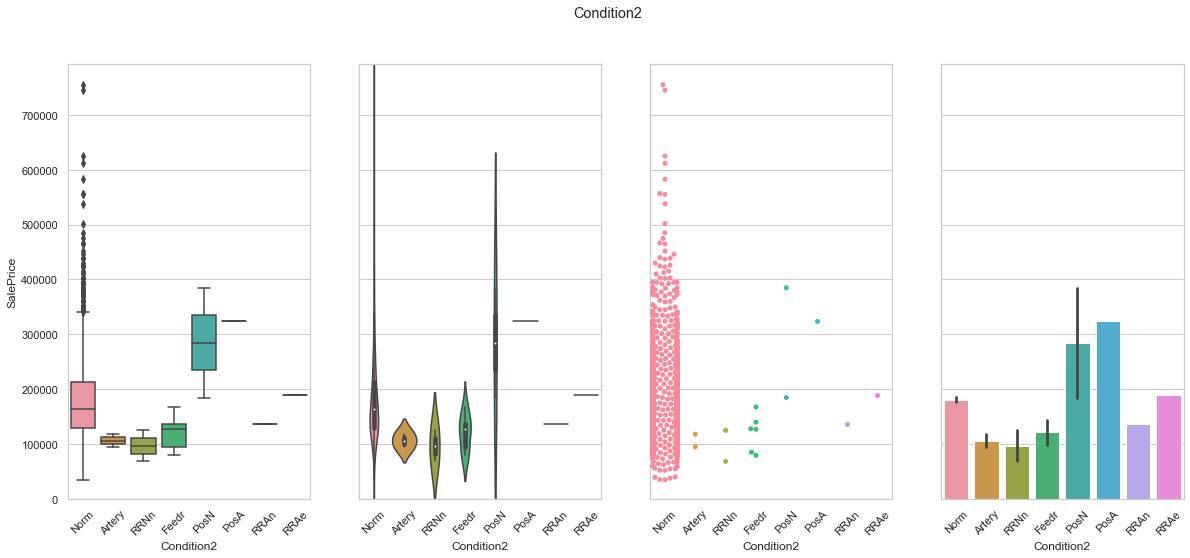
COMMENT

For both features, the data is concentrated into a single class.
The distribution between the two features is similar.

feature = 'LotFrontage'
plot_num_feature_eda(feature)

LotFrontage

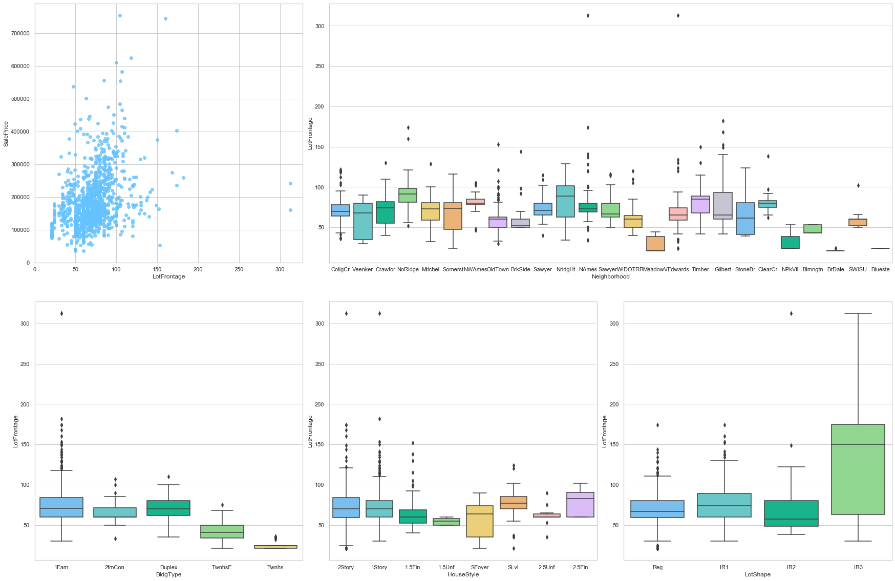
COMMENT

The original set presents a large number of null values.
The neighborhoods and the house type do not seem to play a significant role for this feature.

feature = 'LotArea'
plot_num_feature_eda(feature)

LotArea

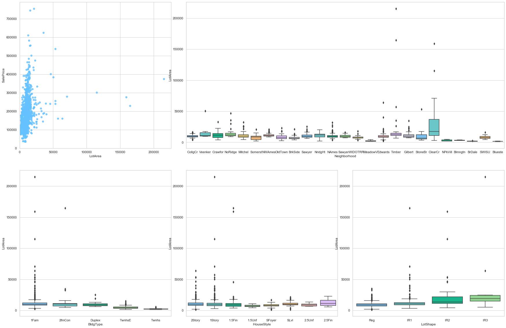
COMMENT

As expected, this feature is strongly positively correlated to the sale price.

feature = 'LotShape'
plot_cat_feature_eda(feature)

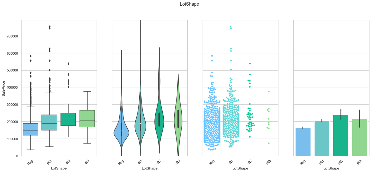
COMMENT

The data is concentrated into two classes.

feature = 'LandContour'
plot_cat_feature_eda(feature)

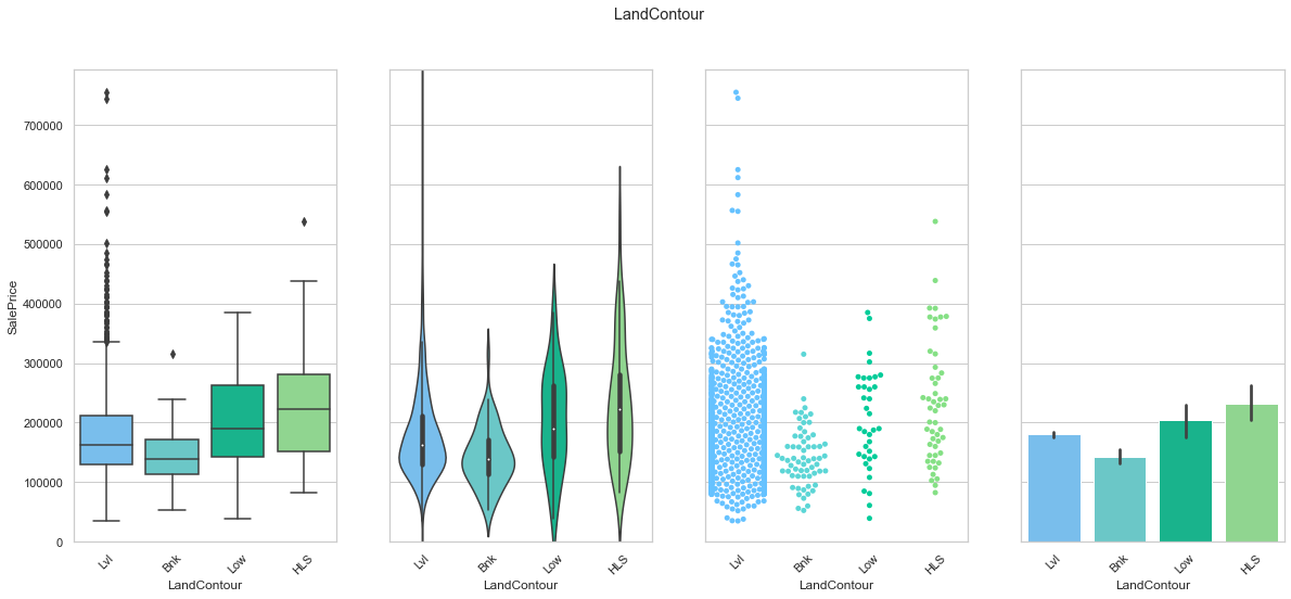
COMMENT

The data is concentrated into a single class.

feature = 'LotConfig'
plot_cat_feature_eda(feature)

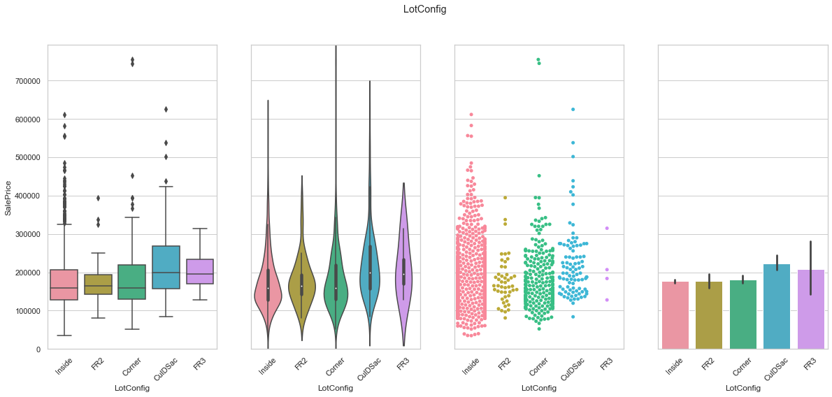
COMMENT

The data is concentrated into three classes.
FR2 and FR3 are merged.

feature = 'LandSlope'
plot_cat_feature_eda(feature)

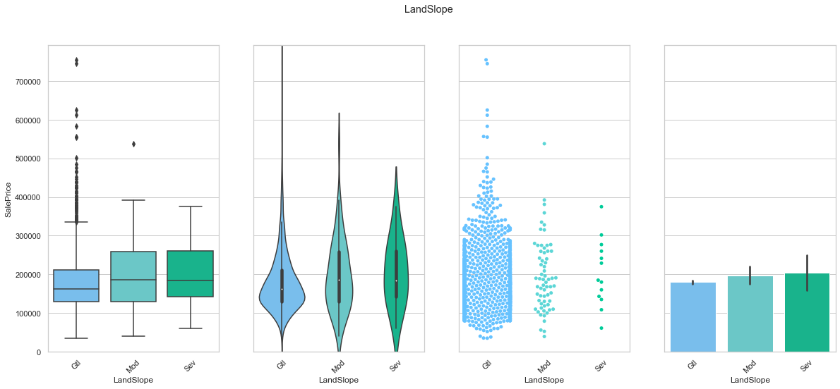
COMMENT

This feature does not have a clear impact on the sale price.

feature = 'Street'
plot_cat_feature_eda(feature)

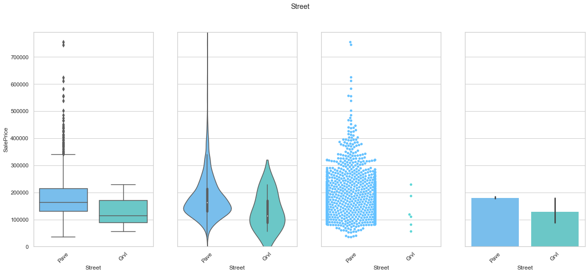
COMMENT

The vast majority of the data is stored under the same class.

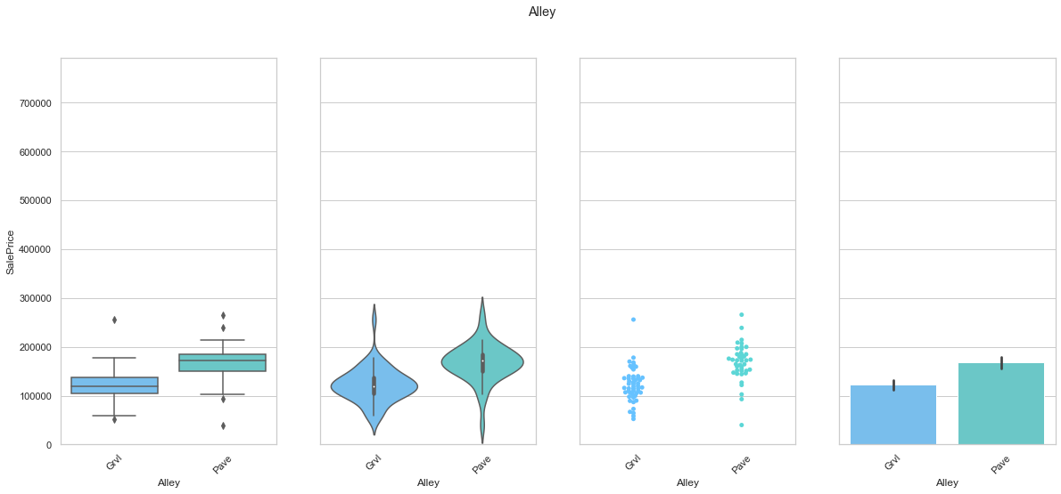
feature = 'Alley'
plot_cat_feature_eda(feature)

COMMENT

There is a slight difference in the sale price between the two classes.

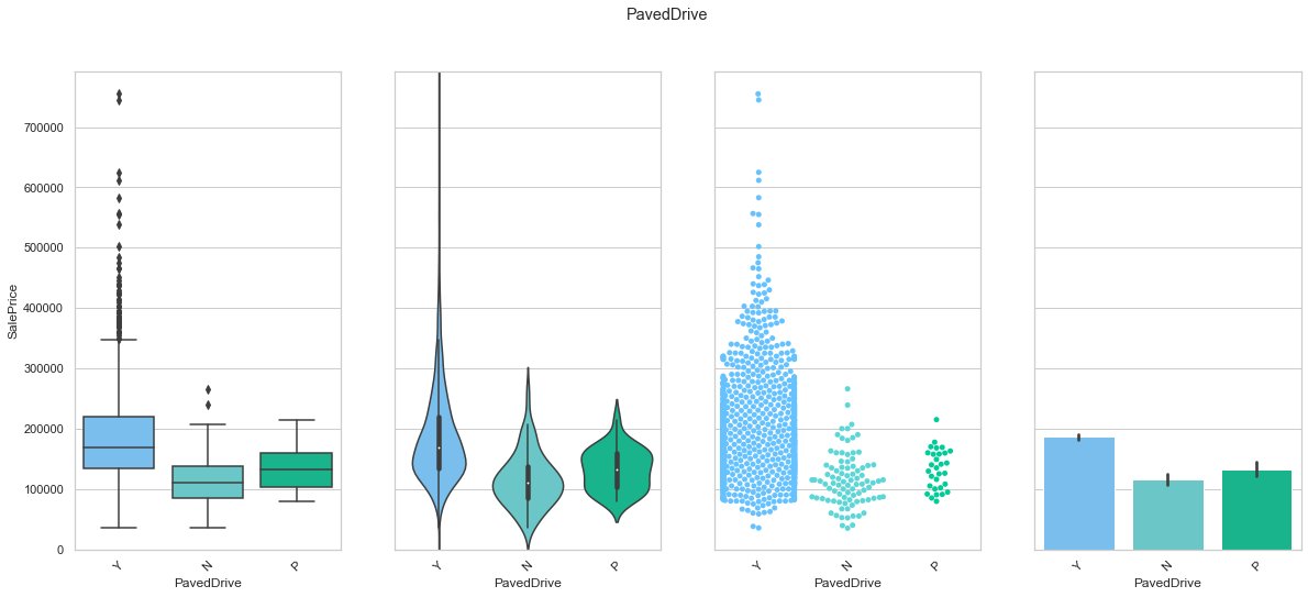
feature = 'PavedDrive'
plot_cat_feature_eda(feature)

COMMENT

Most of the data is contained in the Y class.
There is a slight difference in the sale price between the three classes.

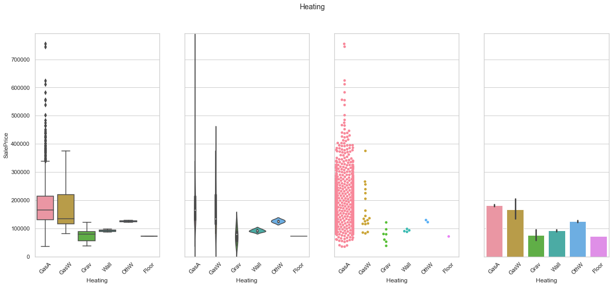
feature = 'Heating'
plot_cat_feature_eda(feature)

COMMENT

The vast majority of the data is contained in the GasA class.

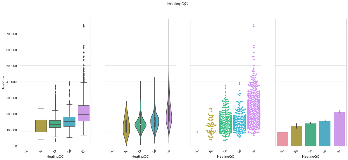
feature = 'HeatingQC'
order=["Po", "Fa", "TA", "Gd", "Ex"]
plot_cat_feature_eda(feature, order)

COMMENT

We were able to find a order that corresponds to an increase in sale price.

feature = 'CentralAir'
plot_cat_feature_eda(feature)

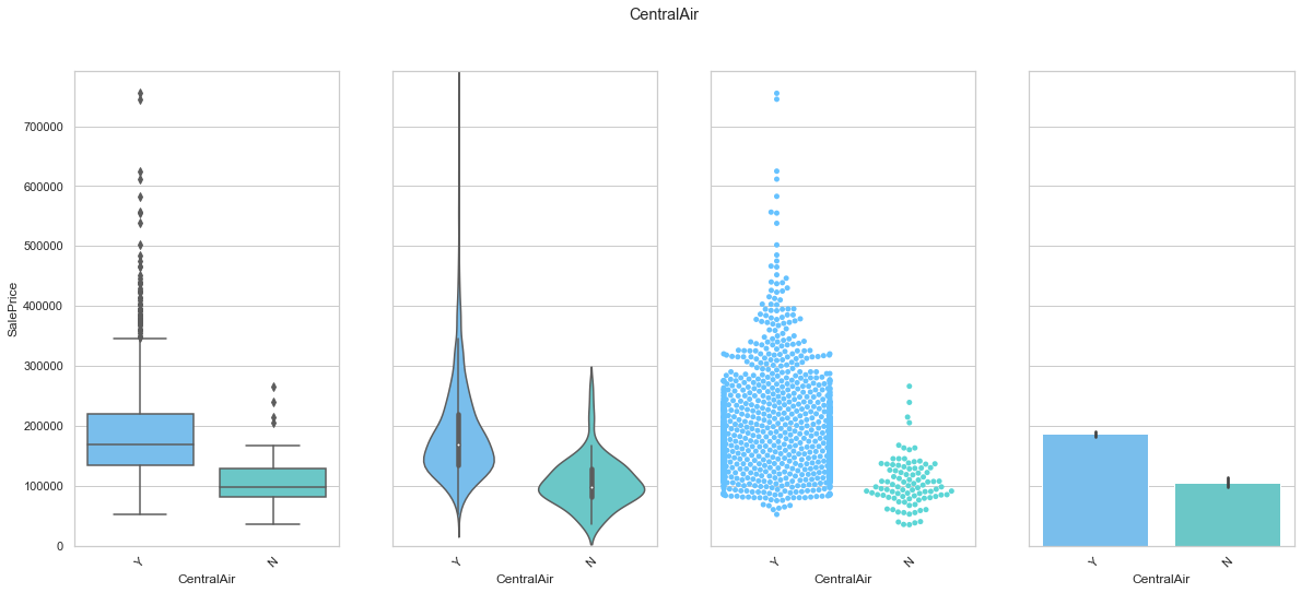
COMMENT

The data is mostly stored under the “Y” class. Since this feature is a boolean feature, we simply map “Y” to the value 1 and “No” to the value 0.

feature = 'Utilities'
plot_cat_feature_eda(feature)

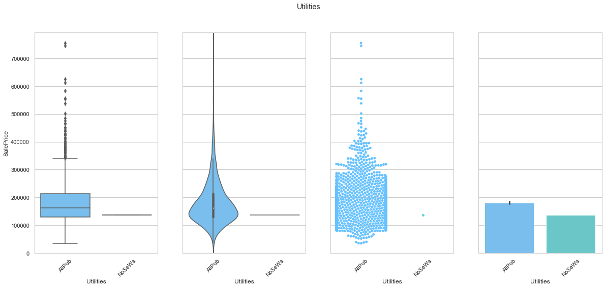
COMMENT

The utilities feature can be dropped since the data is mostly assigned to a single class.

feature = 'Electrical'
plot_cat_feature_eda(feature)

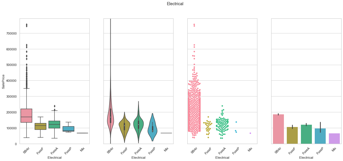
COMMENT

As seen before, the date is mostly contained in a single class.

feature = 'MiscFeature'
plot_cat_feature_eda(feature)

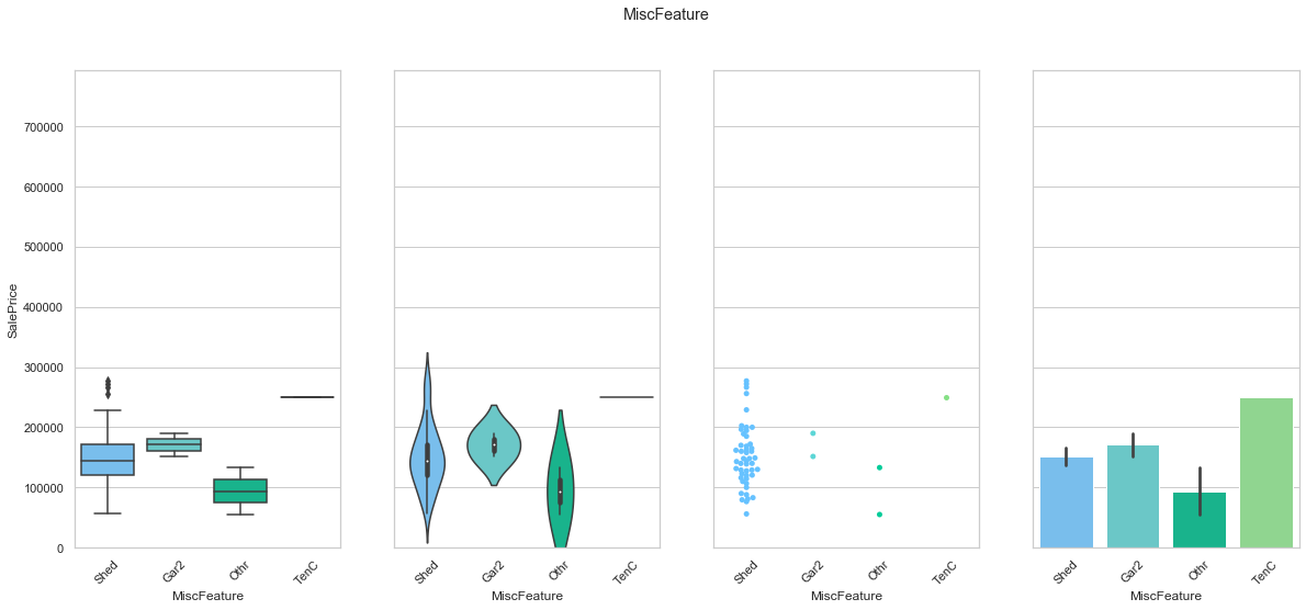
COMMENT

Only a small fraction of the dataset has a MiscFeature assigned.

feature = 'MoSold'
plot_cat_feature_eda(feature)

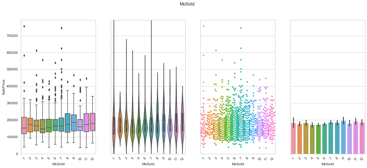
COMMENT

The data is mostly homogeneously distributed although a few months (summer) are more proned to sales.

feature = 'YrSold'
plot_cat_feature_eda(feature)

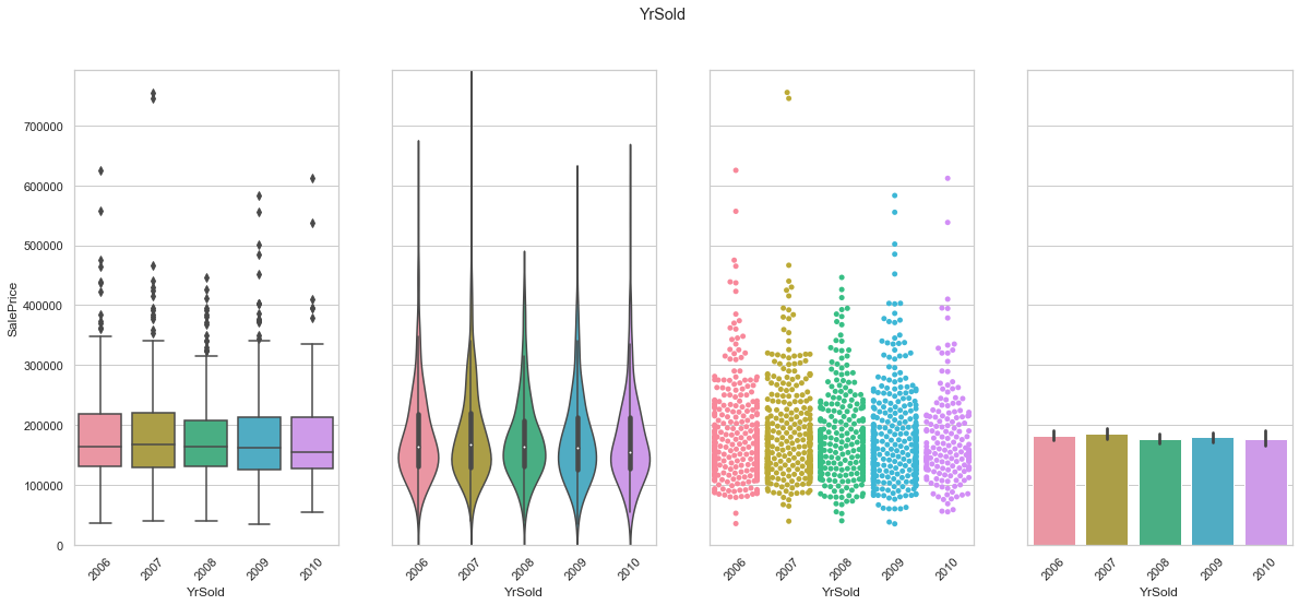
COMMENT

It does not appear to be a large correlation between the year of the sale and the selling price.

feature = 'SaleType'
plot_cat_feature_eda(feature)

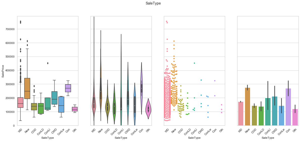
COMMENT

Most of the sales are contained in the “WD” features.
The “New” feature has an higher average sale price.

feature = 'SaleCondition'
plot_cat_feature_eda(feature)

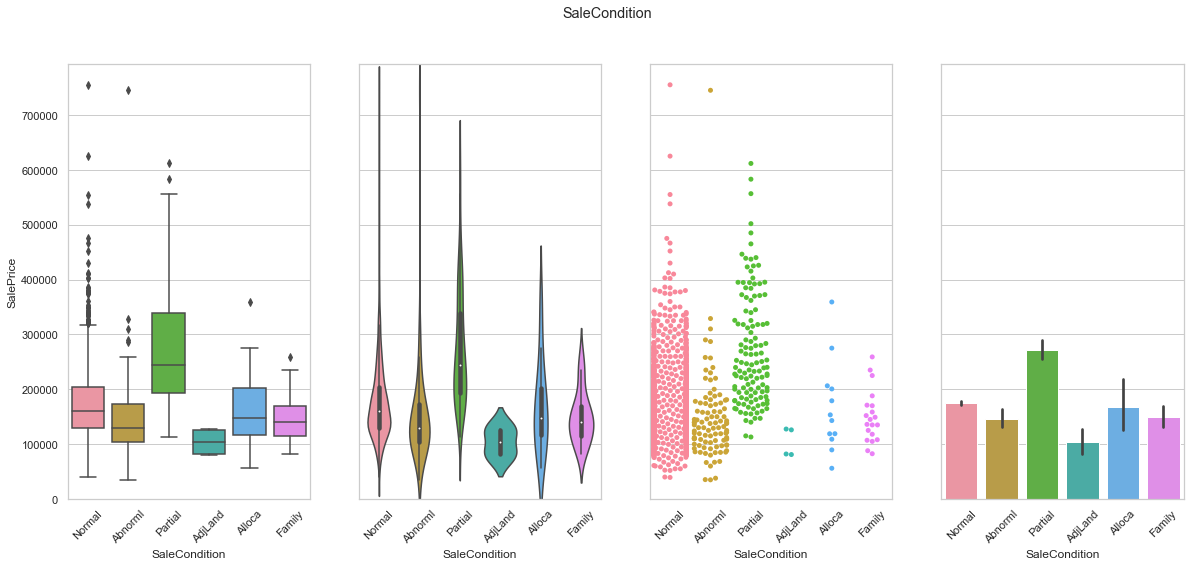
COMMENT

Most of the data is contained in the “Normal” class.
The sale condition seems to have a significant impact on the sale price as the sale price for each class differs from the ones of the other classes.

3. Pre-Processing

The first step consists of isolating the target label from the dataset.

# clean import
train = pd.read_csv('./data/train.csv')
test = pd.read_csv('./data/test.csv')

# isolate ID's
test_id = test['Id']
train_id = train['Id']

# remove ID from sets
train = train.drop(['Id'], axis=1)
test = test.drop(['Id'], axis=1)

print("Train:", train.shape)
print("Test", test.shape)

Train: (1460, 80)
Test (1459, 79)

We have previously seen that the sale price was not normally distributed and that it required a transformation.

train['SalePrice'] = np.log1p(train['SalePrice'])

# Deleting outliers
train = train[train.GrLivArea < 4500]
train_end = train.shape[0]
train.reset_index(drop=True, inplace=True)

y_train = train['SalePrice']
train = train.drop(['SalePrice'], axis=1)

full_set = pd.concat([train, test]).reset_index(drop=True)
print('Shape of the entire dataset is {}'.format(full_set.shape))

Shape of the entire dataset is (2917, 79)

# plot new distribution after transformation
mu, sigma = norm.fit(y_train)
sns.distplot(y_train, fit=norm)
plt.legend(['Normal distribution ($$\mu=$$ {:.2f} and $$\sigma=$$ {:.2f} )'.format(mu, sigma)], loc = 'best')
plt.ylabel('Frequency')
plt.title('Histogram of SalePrice');

fig = plt.figure()
res = probplot(y, plot=plt);

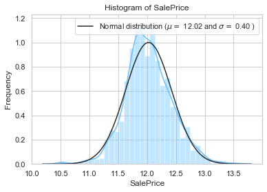
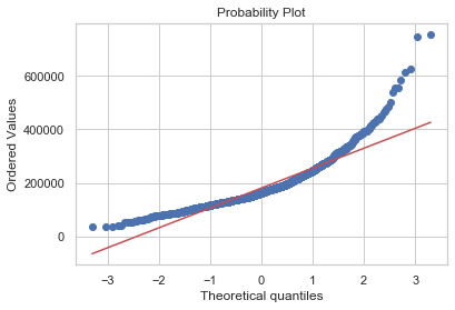
As shown above, the transformed label has a distribution closer to the normal distribution. The tails of the sale price features are still larger but at least, we have a better fit for our model.

Identify the list of features with missing values:

nulls = full_set.isnull().sum(axis=0)
nulls[nulls > 0].sort_values(ascending=False)

PoolQC          2908
MiscFeature     2812
Alley           2719
Fence           2346
FireplaceQu     1420
LotFrontage      486
GarageFinish     159
GarageYrBlt      159
GarageQual       159
GarageCond       159
GarageType       157
BsmtExposure      82
BsmtCond          82
BsmtQual          81
BsmtFinType2      80
BsmtFinType1      79
MasVnrType        24
MasVnrArea        23
MSZoning           4
BsmtFullBath       2
BsmtHalfBath       2
Utilities          2
Functional         2
Exterior2nd        1
Exterior1st        1
SaleType           1
BsmtFinSF1         1
BsmtFinSF2         1
BsmtUnfSF          1
Electrical         1
KitchenQual        1
GarageCars         1
GarageArea         1
TotalBsmtSF        1
dtype: int64

We previously saw that our features have distributions that cannot be approximated by the normal distribution. We compute the skew of each feature to see which ones can be corrected.

# Isolate numerical feature names
numerical = full_set.dtypes[full_set.dtypes != 'object'].index

#compute skew and sort
skewness = full_set[numerical].apply(lambda x: skew(x.dropna())).sort_values(ascending=False)
skewness

MiscVal          21.939672
PoolArea         17.688664
LotArea          13.109495
LowQualFinSF     12.084539
3SsnPorch        11.372080
KitchenAbvGr      4.300550
BsmtFinSF2        4.143683
EnclosedPorch     4.002344
ScreenPorch       3.945101
BsmtHalfBath      3.928397
MasVnrArea        2.609358
OpenPorchSF       2.529358
WoodDeckSF        1.844792
MSSubClass        1.375131
1stFlrSF          1.257286
LotFrontage       1.121322
GrLivArea         1.068750
BsmtFinSF1        0.980283
BsmtUnfSF         0.919699
2ndFlrSF          0.861556
TotRmsAbvGrd      0.749232
Fireplaces        0.725278
HalfBath          0.696666
TotalBsmtSF       0.676200
BsmtFullBath      0.621322
OverallCond       0.569314
BedroomAbvGr      0.326568
GarageArea        0.218752
MoSold            0.197345
OverallQual       0.189591
FullBath          0.165514
YrSold            0.131996
GarageCars       -0.217977
GarageYrBlt      -0.380955
YearRemodAdd     -0.450134
YearBuilt        -0.599194
dtype: float64

The Box-Cox transformation can be used to adjust feature with high skewness. Several values of the parameter lambda are tested and a threshold of 0.5 is used to determine which feature needs to be transformed.

def FeatureEngineering(input_df, train_df, threshold=0.50):
    
    df = input_df.copy()
    
    # Change data-type
    df['MSSubClass'] = df['MSSubClass'].apply(str)
    df['YrSold'] = df['YrSold'].astype(str)
    df['MoSold'] = df['MoSold'].astype(str)
    
    # Fill empty records with generic class
    df['Functional'] = df['Functional'].fillna('Typ') 
    df['Electrical'] = df['Electrical'].fillna("SBrkr") 
    df['KitchenQual'] = df['KitchenQual'].fillna("TA") 
    
    # Fill empty records with new None class
    df["PoolQC"] = df["PoolQC"].fillna("None")
    
    df["GarageType"] = df["GarageType"].fillna("None")
    df["GarageFinish"] = df["GarageFinish"].fillna("None")
    df["GarageQual"] = df["GarageQual"].fillna("None")
    df["GarageCond"] = df["GarageCond"].fillna("None")
    
    df["BsmtQual"] = df["BsmtQual"].fillna("None")
    df["BsmtCond"] = df["BsmtCond"].fillna("None")
    df["BsmtExposure"] = df["BsmtExposure"].fillna("None")    
    
    # Fill records with mode
    df['Exterior1st'] = df['Exterior1st'].fillna(df['Exterior1st'].mode()[0]) 
    df['Exterior2nd'] = df['Exterior2nd'].fillna(df['Exterior2nd'].mode()[0])
    df['SaleType'] = df['SaleType'].fillna(df['SaleType'].mode()[0])
    
    # Fill numerical feature with 0
    df["GarageYrBlt"] = df["GarageYrBlt"].fillna(0)
    df["GarageArea"] = df["GarageArea"].fillna(0)
    df["GarageCars"] = df["GarageCars"].fillna(0)
    
    # Fill connected features using groups
    df['MSZoning'] = df.groupby('MSSubClass')['MSZoning'].transform(lambda x: x.fillna(x.mode()[0]))
           
    # Process remaining features
    objects = []
    for col in df.columns:
        if df[col].dtype == object:
            objects.append(col)
    df.update(df[objects].fillna('None')) 
    
    # Fill connected features using groups
    df['LotFrontage'] = df.groupby('Neighborhood')['LotFrontage'].transform(lambda x: x.fillna(x.median()))
    
    # Process remaining features
    numeric_dtypes = ['int16', 'int32', 'int64', 'float16', 'float32', 'float64']
    numeric_features = []
    for col in df.columns:
        if df[col].dtype in numeric_dtypes:
            numeric_features.append(col)   
    df.update(df[numeric_features].fillna(0)) 
    
    # drop features
    df = df.drop(['Utilities', 'Street', 'PoolQC',], axis=1)
        
    # Use log of data to reduce the impact of outliers
    continuous_features = []
    
    for col in df.columns:
        if df[col].dtype in numeric_dtypes:
            continuous_features.append(col)
    
    categorical_features = [col for col in df.columns if col not in continuous_features]
    
    # Skewness correction
    skewness = df[continuous_features].apply(lambda x: skew(x.dropna())).sort_values(ascending=False)
    boxcox_features = skewness[skewness>threshold].index
    
    for col in boxcox_features:
        df[col] = boxcox1p(df[col], boxcox_normmax(df[col] + 1))
                
    # New features
    df['TotalSF'] = df['TotalBsmtSF'] + df['1stFlrSF'] + df['2ndFlrSF']
    df['YrBltAndRemod']=df['YearBuilt']+df['YearRemodAdd']
    
    df['Total_sqr_footage'] = (df['BsmtFinSF1'] + df['BsmtFinSF2'] +
                                 df['1stFlrSF'] + df['2ndFlrSF'])
    
    df['Total_Bathrooms'] = (df['FullBath'] + (0.5 * df['HalfBath']) +
                               df['BsmtFullBath'] + (0.5 * df['BsmtHalfBath']))
    
    df['Total_porch_sf'] = (df['OpenPorchSF'] + df['3SsnPorch'] +
                              df['EnclosedPorch'] + df['ScreenPorch'] +
                              df['WoodDeckSF'])
    
    df['haspool'] = df['PoolArea'].apply(lambda x: 1 if x > 0 else 0)
    df['has2ndfloor'] = df['2ndFlrSF'].apply(lambda x: 1 if x > 0 else 0)
    df['hasgarage'] = df['GarageArea'].apply(lambda x: 1 if x > 0 else 0)
    df['hasbsmt'] = df['TotalBsmtSF'].apply(lambda x: 1 if x > 0 else 0)
    df['hasfireplace'] = df['Fireplaces'].apply(lambda x: 1 if x > 0 else 0)
        
    # generate dummy features
    df = pd.get_dummies(df).reset_index(drop=True)
    
    # filtering data by removing columns made almost entirely of one value
    overfit = []
    
    for i in df.columns:
        counts = df[i].value_counts()
        most_common = counts.iloc[0]
        if most_common / len(df) * 100 > 99.94:
            overfit.append(i)
    
    overfit.append('MSZoning_C (all)')
    df = df.drop(overfit, axis=1)
        
    return df

# transform entire dataset
transformed_full_set = FeatureEngineering(full_set, train)
print(transformed_full_set.shape)

(2917, 321)

# Split full dataset using train and test set
train = transformed_full_set.iloc[:train_end, :]
test  = transformed_full_set.iloc[train_end:, :]

print('train', train.shape, 'y_train', y_train.shape, 'test',test.shape)

train (1458, 321) y_train (1458,) test (1459, 321)

The training and test sets are ready to be used to train our models.

4. Models

4.1. Benchmarking

The prediction of the sale price is a regression problem. Our strategy will consists of performing a cross-validation on the train model (using a K-fold approach). The initial step consists of training a set of regression models (using default hyper-parameters). The objectives of this first training step are to select and identify models with good performances. These models can then be further trained.
The following models are used during the first training phase: Ridge Regression

Lasso Regression
ElasticNet Regression
KNN Reggressor
Bayesian Regressor
Decision Tree
SVM
Gradient Boosting
ExtraTree
Random Forest

# scaler
robust = RobustScaler()

# scale training set
train_normalized = robust.fit_transform(train)

# scalre test set
test_normalized = robust.transform(test)

train_normalized.shape

(1458, 321)

models = [Lasso(), ElasticNet(), KNeighborsRegressor(),
          BayesianRidge(), DecisionTreeRegressor(), SVR(),
          GradientBoostingRegressor(), ExtraTreesRegressor(), RandomForestRegressor(),
          LGBMRegressor(), XGBRegressor(objective='reg:squarederror')]

kfolds = KFold(n_splits=10, shuffle=True, random_state=42)

# results summary
summary_cols = ['Model', 'Parameters (Pre)', 'CV_results', 'CV_mean', 'CV_std']
summary_df = pd.DataFrame(columns=summary_cols)

for idx, algo in enumerate(models):
    
    # identify the model
    name = algo.__class__.__name__
    summary_df.loc[idx,'Model'] = name
    summary_df.loc[idx,'Parameters (Pre)'] = str(algo.get_params())
      
    # cross-valudation
    scores = cross_val_score(algo, train_normalized, y_train, cv=5, scoring='neg_mean_squared_error')
    
    # compute metrics   
    summary_df.loc[idx,'CV_results'] = "RMSE: %0.2f (+/- %0.3f)" % (scores.mean(), scores.std() * 2)
    summary_df.loc[idx,'CV_mean'] = -scores.mean()
    summary_df.loc[idx,'CV_std'] = scores.std() * 2
    print(algo.__class__.__name__, 'trained...')

#summary_df['Training accuracy (Pre)'] = summary_df['Training accuracy (Pre)'].apply(lambda x: round(x, decimals))
#summary_df['Testing accuracy (Pre)'] = summary_df['Testing accuracy (Pre)'].apply(lambda x: round(x, decimals))

print("\n\nSummary without hyper-parameter tuning:")

summary_df = summary_df.sort_values(['CV_mean'])
summary_df.reset_index(drop=True)

Lasso trained...
ElasticNet trained...
KNeighborsRegressor trained...
BayesianRidge trained...
DecisionTreeRegressor trained...
SVR trained...
GradientBoostingRegressor trained...
ExtraTreesRegressor trained...
RandomForestRegressor trained...
LGBMRegressor trained...
XGBRegressor trained...


Summary without hyper-parameter tuning:

	Model	Parameters (Pre)	CV_results	CV_mean	CV_std
0	BayesianRidge	{'alpha_1': 1e-06, 'alpha_2': 1e-06, 'compute_...	RMSE: -0.01 (+/- 0.003)	0.0128691	0.00283413
1	XGBRegressor	{'base_score': 0.5, 'booster': 'gbtree', 'cols...	RMSE: -0.02 (+/- 0.003)	0.015208	0.00251774
2	GradientBoostingRegressor	{'alpha': 0.9, 'criterion': 'friedman_mse', 'i...	RMSE: -0.02 (+/- 0.002)	0.0153384	0.00219738
3	SVR	{'C': 1.0, 'cache_size': 200, 'coef0': 0.0, 'd...	RMSE: -0.02 (+/- 0.004)	0.0158596	0.00404555
4	LGBMRegressor	{'boosting_type': 'gbdt', 'class_weight': None...	RMSE: -0.02 (+/- 0.003)	0.0158715	0.00270137
5	ExtraTreesRegressor	{'bootstrap': False, 'criterion': 'mse', 'max_...	RMSE: -0.02 (+/- 0.006)	0.0214468	0.00565928
6	RandomForestRegressor	{'bootstrap': True, 'criterion': 'mse', 'max_d...	RMSE: -0.02 (+/- 0.004)	0.0219718	0.00445915
7	KNeighborsRegressor	{'algorithm': 'auto', 'leaf_size': 30, 'metric...	RMSE: -0.03 (+/- 0.005)	0.0333655	0.00541219
8	DecisionTreeRegressor	{'criterion': 'mse', 'max_depth': None, 'max_f...	RMSE: -0.04 (+/- 0.010)	0.038983	0.0100607
9	ElasticNet	{'alpha': 1.0, 'copy_X': True, 'fit_intercept'...	RMSE: -0.14 (+/- 0.022)	0.142879	0.0217675
10	Lasso	{'alpha': 1.0, 'copy_X': True, 'fit_intercept'...	RMSE: -0.15 (+/- 0.025)	0.149546	0.0248788

# plot results
fig, ax = plt.subplots(figsize=(12,12))
g = sns.barplot("CV_mean",
                "Model",
                data = summary_df,
                palette="Set3",
                orient = "h",
                **{'xerr':summary_df['CV_std'].values})
g.set_xlabel("Mean Accuracy")
g = g.set_title("Cross validation scores")

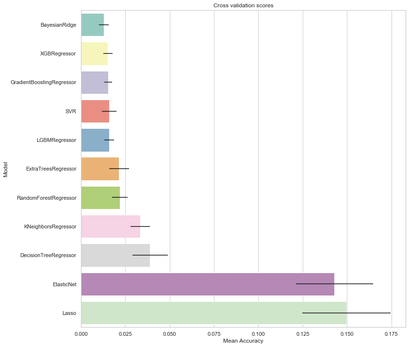
The models tested above are sorted by RMSE on the cross-validation fold. The top 9 lead to relatively low RMSE. We can now inspect feature importances.

4.2. Feature Importances

# create an DecisionTreeRegressor
model = DecisionTreeRegressor()

# fit the model
model.fit(train_normalized, y_train)

# sort features by importances
indices = np.argsort(model.feature_importances_)[::-1]
n_feature = len(model.feature_importances_[model.feature_importances_>0])

print(n_feature," features are important.")

209  features are important.

# plot the feature importances
top_n = 20

indices = indices[0:top_n]
plt.subplots(figsize=(20,20))

g = sns.barplot(y=train.columns[indices], x=model.feature_importances_[indices], palette = mycols)
g.set_xlabel('feature importance')
g.set_ylabel('feature')
g.set_title('DecisionTreeRegressor (Top {} features)'.format(top_n))
g.tick_params(labelsize=15);

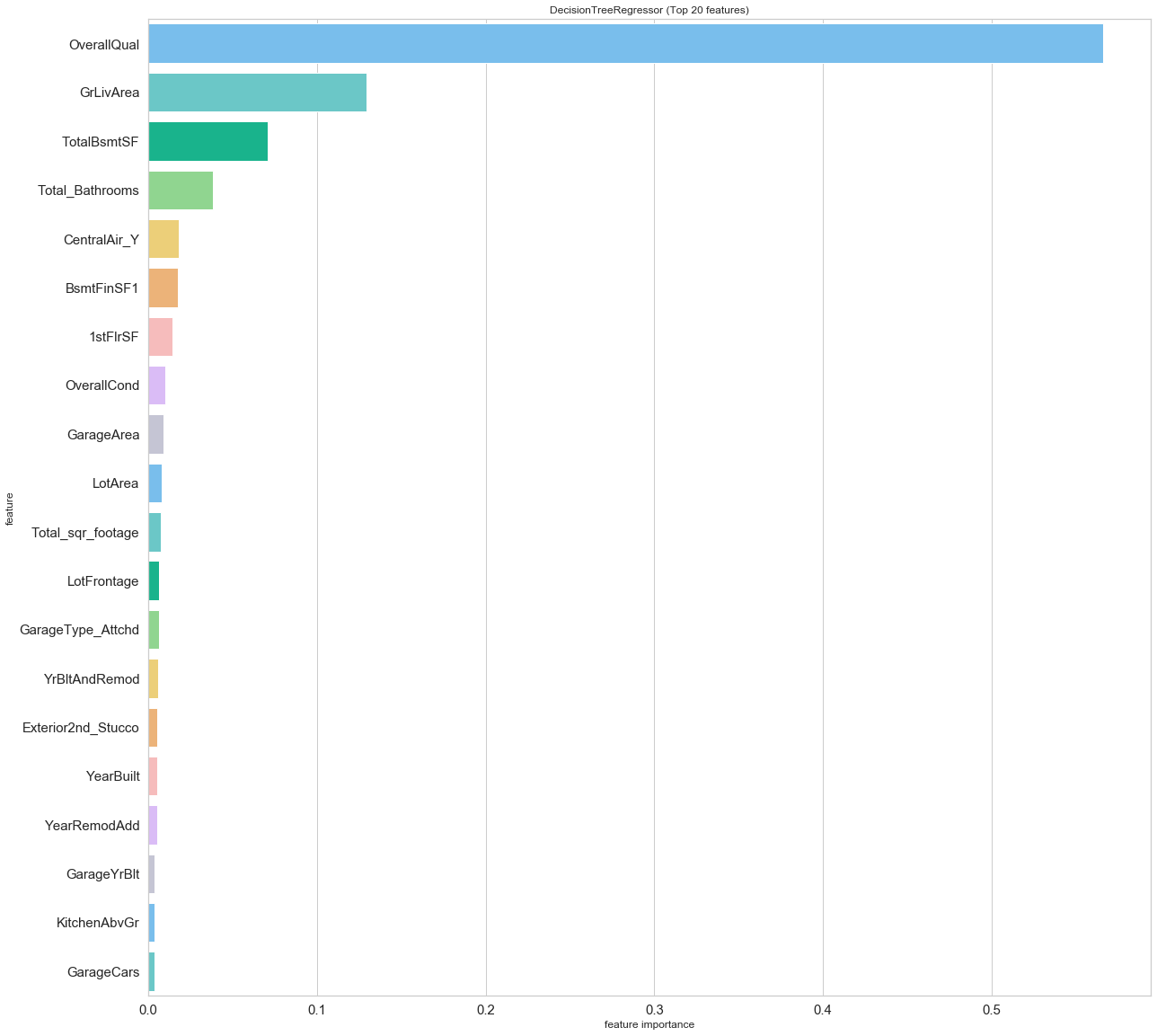
As expected, some of the fundamental real-estate features appear as the most important, such as the overall quality, the size of the living area, the number of bathrooms.

4.3. Result Correlation and Model Behaviors

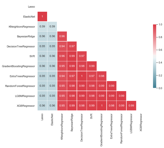
Before performing any ensembling, we must evaluate the correlation between the predictions of our models. Indeed, the ensembling works best when the selected models lead to uncorrelated predictions.

summary_cols = ['Model', 'Parameters (Pre)', 'CV results', 'CV mean', 'CV std']
summary_df = pd.DataFrame(columns=summary_cols)

predictions_df = pd.DataFrame()

for idx, algo in enumerate(models):
    algo.fit(train_normalized, y_train)
    predictions = pd.Series(algo.predict(train_normalized))
    
    predictions_df[algo.__class__.__name__] = predictions

# Compute the correlation matrix
corr = predictions_df.corr()

# Generate a mask for the upper triangle
mask = np.zeros_like(corr, dtype=np.bool)
mask[np.triu_indices_from(mask)] = True

# Set up the matplotlib figure
f, ax = plt.subplots(figsize=(10, 12))

# Generate a custom diverging colormap
cmap = sns.diverging_palette(220, 10, as_cmap=True)

# Draw the heatmap with the mask and correct aspect ratio
sns.heatmap(corr, mask=mask, cmap=cmap, vmax=1.0,vmin=0.0, center=1/2.,annot=True,
            square=True, linewidths=.5, cbar_kws={"shrink": .4});

4.4. Ensembling

Now that the basic models have been tested and their results assessed, an ensemble of tuned model is created. First, each one of the selected model has its hyperparameters tuned.

Each of the model is trained using a k-fold validation method (using 10 folds).

# create k-fold
kfolds = KFold(n_splits=10, shuffle=True, random_state=42)

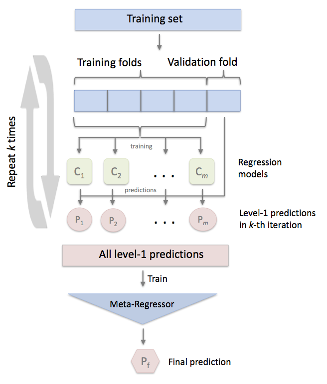
In addition, we create a stacking cross-validation regressor. This ensemble technique consists of combining several regressors, train them using CV, add the predictions to the dataset as new features and train a meta-regressor with the new dataset.

# setup models   

# Ridge parameters
alphas_alt = [14.5, 14.6, 14.7, 14.8, 14.9, 15, 15.1, 15.2, 15.3, 15.4, 15.5]

# Lasso parameters
alphas2 = [5e-05, 0.0001, 0.0002, 0.0003, 0.0004, 0.0005, 0.0006, 0.0007, 0.0008]

# ElasticNet
e_alphas = [0.0001, 0.0002, 0.0003, 0.0004, 0.0005, 0.0006, 0.0007]
e_l1ratio = [0.8, 0.85, 0.9, 0.95, 0.99, 1]

ridge = RidgeCV(alphas=alphas_alt, cv=kfolds)

lasso = LassoCV(max_iter=1e7, alphas=alphas2, random_state=42, cv=kfolds)

elasticnet = ElasticNetCV(max_iter=1e7, alphas=e_alphas, cv=kfolds, l1_ratio=e_l1ratio)
                                        
svr = SVR(C= 20, epsilon= 0.008, gamma=0.0003,)


gbr = GradientBoostingRegressor(n_estimators=3000, learning_rate=0.05,
                                   max_depth=4, max_features='sqrt',
                                   min_samples_leaf=15, min_samples_split=10, 
                                   loss='huber', random_state =42)
                                   
lightgbm = LGBMRegressor(objective='regression', 
                                       num_leaves=4,
                                       learning_rate=0.01, 
                                       n_estimators=5000,
                                       max_bin=200, 
                                       bagging_fraction=0.75,
                                       bagging_freq=5, 
                                       bagging_seed=7,
                                       feature_fraction=0.2,
                                       feature_fraction_seed=7,
                                       verbose=-1)
                                       
xgboost = XGBRegressor(learning_rate=0.01, n_estimators=3460,
                                     max_depth=3, min_child_weight=0,
                                     gamma=0, subsample=0.7,
                                     colsample_bytree=0.7,
                                     nthread=-1,
                                     scale_pos_weight=1, seed=27,
                                     objective='reg:squarederror',
                                     reg_alpha=0.00006)

stack_gen = StackingCVRegressor(regressors=(ridge, lasso, elasticnet,
                                            gbr, xgboost, lightgbm),
                                meta_regressor=xgboost,
                                use_features_in_secondary=True)

Once the tunable models have been defined, they are trained using the training set.

ridge_model_full_data = ridge.fit(train_normalized, y_train)
print('Ridge trained...')
lasso_model_full_data = lasso.fit(train_normalized, y_train)
print('Lasso trained...')
elastic_model_full_data = elasticnet.fit(train_normalized, y_train)
print('Elastic trained...')
svr_model_full_data = svr.fit(train_normalized, y_train)
print('SVR trained...')
gbr_model_full_data = gbr.fit(train_normalized, y_train)
print('GBR trained...')
lgb_model_full_data = lightgbm.fit(train_normalized, y_train)
print('LGB trained...')
xgb_model_full_data = xgboost.fit(train_normalized, y_train)
print('XGB trained...')
stack_gen_model = stack_gen.fit(train_normalized, y_train)
print('Stack trained...')

Ridge trained...
Lasso trained...
Elastic trained...
SVR trained...
GBR trained...
LGB trained...
XGB trained...
Stack trained...

The Kaggle competition defines the key metric as the root-mean-squared error. Since our data has been transformed using a log function, our corresponding metric is the root-mean-squared logarithmic error (RMSLE).

# rmsle
def rmsle(y, y_pred):
    return np.sqrt(mean_squared_error(y, y_pred))


# scoring function
def cv_rmse(model, X=train_normalized, y=y_train):
    rmse = np.sqrt(-cross_val_score(model, X, y,
                                    scoring="neg_mean_squared_error",
                                    cv=kfolds))
    return (rmse)

The RMSLE (means and standard deviation) is computed for each of the tuned model.

score = cv_rmse(ridge)
print("Kernel Ridge score: {:.4f} ({:.4f})".format(score.mean(), score.std()))

score = cv_rmse(lasso)
print("Lasso score: {:.4f} ({:.4f})".format(score.mean(), score.std()),)

score = cv_rmse(elasticnet)
print("ElasticNet score: {:.4f} ({:.4f})".format(score.mean(), score.std()))

score = cv_rmse(svr)
print("SVR score: {:.4f} ({:.4f})".format(score.mean(), score.std()))

score = cv_rmse(lightgbm)
print("Lightgbm score: {:.4f} ({:.4f})".format(score.mean(), score.std()))

score = cv_rmse(gbr)
print("GradientBoosting score: {:.4f} ({:.4f})".format(score.mean(), score.std()))

score = cv_rmse(xgboost)
print("Xgboost score: {:.4f} ({:.4f})".format(score.mean(), score.std()))

score = cv_rmse(stack_gen)
print("Stack score: {:.4f} ({:.4f})".format(score.mean(), score.std()))

Kernel Ridge score: 0.1100 (0.0166)
Lasso score: 0.1104 (0.0165)
ElasticNet score: 0.1103 (0.0165)
SVR score: 0.1091 (0.0185)
Lightgbm score: 0.1139 (0.0156)
GradientBoosting score: 0.1135 (0.0152)
Xgboost score: 0.1155 (0.0165)
Stack score: 0.1133 (0.0143)

We now create a new stack combining our models. The new model consists of a simple linear combination of the previous model. More emphasis is put on the stack model. This is done by assigning a larger weight to this model. The definition of the weights of the model are based on trial-and-error. We start with 0.1 for all model except for the stack (0.3 weight).

def blend_models_predict(X):
    return (
        (0.15 * ridge_model_full_data.predict(X)) + \
        (0.1 * lasso_model_full_data.predict(X)) + \
        
        (0.1 * elastic_model_full_data.predict(X)) + \
        (0.1 * svr_model_full_data.predict(X)) + \
            
        (0.1 * lgb_model_full_data.predict(X)) + \
        (0.1 * gbr_model_full_data.predict(X)) + \
            
        (0.1 * xgb_model_full_data.predict(X)) + \
        (0.25 * stack_gen_model.predict(np.array(X)))
    )
            
print('RMSLE score on train data:')
print(rmsle(y_train, blend_models_predict(train_normalized)))

RMSLE score on train data:
0.0660008865648205

4.5. Fine Tuning

The final assessment of our model is based on the residual distribution. The sale prices from the training set are compared to the predicted sale prices. The goal is to determine if the outliers of the training set led to a bias error.

# predictions
y_pred = np.floor(np.expm1(blend_models_predict(train_normalized)))
y_train_real = np.floor(np.floor(np.expm1(y_train)))

# create figure
fig, axs = plt.subplots(1, 2, figsize=(16,8))

# set axis labels
axs[0].set_xlabel('Sale Price - Real Values')
axs[0].set_ylabel('Sale Price - Predicted Values')

# plot real vs. predicted
axs[0].scatter(y_train_real, y_pred, marker='.', label='blend model')

# plot x=y for comparison
x_range = [np.min(y_train_real), np.max(y_train_real)]
axs[0].plot(x_range, x_range, c='k', label="x=y")
axs[0].legend()

# plot residuals
axs[1].scatter(y_train_real, y_pred-y_train_real, marker='.')
axs[1].set_xlabel('Sale Price - Real Values')
axs[1].set_ylabel('Sale Price - Residuals');

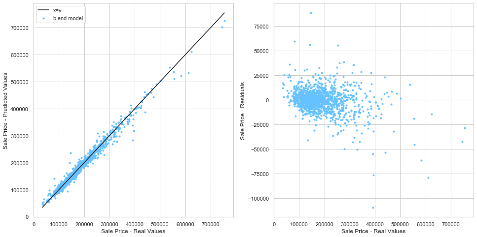
From the above plot, it can be seen that the model tends to under-estimate the price of expensive houses.

In order to re-scale these extreme cases, we group the data by quantiles of the real sale prices. We then inspect the ratio between the predicted values and the real values (grouped by quantiles).

# create residual dataframe
residuals = pd.DataFrame({'real_values':y_train_real, 'pred_values':y_pred, 'residuals':y_pred-y_train_real})

# compute residual quantiles
residuals['quantile_range'] = pd.qcut(residuals['real_values'], q=20)

# compute middle value for each quantile
residuals['middle'] = residuals['quantile_range'].apply(lambda x: (x.left+x.right)/2.).astype(float)

# compute ratio between residual value and quantile mid value
residuals['ratio_res_mid'] = residuals['residuals'] / residuals['middle']

# compute the ratio between the predicted value and the quantile mid value 
residuals['ratio_pred_mid'] = residuals['pred_values'] / residuals['real_values'] 

residuals.head()

	real_values	pred_values	residuals	quantile_range	middle	ratio_res_mid	ratio_pred_mid
0	208499.0	207203.0	-1296.0	(198859.1, 214000.0]	206429.550	-0.006278	0.993784
1	181500.0	187525.0	6025.0	(179239.8, 187500.0]	183369.900	0.032857	1.033196
2	223500.0	214092.0	-9408.0	(214000.0, 230000.0]	222000.000	-0.042378	0.957906
3	139999.0	157285.0	17286.0	(135500.0, 140959.05]	138229.525	0.125053	1.123472
4	249999.0	283155.0	33156.0	(230000.0, 249999.0]	239999.500	0.138150	1.132625

series = residuals.groupby(['quantile_range']).mean()['ratio_pred_mid'].sort_index(ascending=True)
print(series);

quantile_range
(34898.999, 87999.0]     1.095946
(87999.0, 106424.0]      1.019554
(106424.0, 114999.0]     1.004174
(114999.0, 124000.0]     1.001567
(124000.0, 129925.0]     0.999571
(129925.0, 135500.0]     1.001819
(135500.0, 140959.05]    0.997909
(140959.05, 146999.0]    1.007797
(146999.0, 155000.0]     0.993213
(155000.0, 162999.0]     0.993089
(162999.0, 172499.0]     0.997316
(172499.0, 179239.8]     0.995843
(179239.8, 187500.0]     1.011027
(187500.0, 198859.1]     1.004864
(198859.1, 214000.0]     1.001532
(214000.0, 230000.0]     0.994265
(230000.0, 249999.0]     0.996978
(249999.0, 278000.0]     0.988132
(278000.0, 326300.0]     0.991095
(326300.0, 755000.0]     0.968056
Name: ratio_pred_mid, dtype: float64

fig, ax = plt.subplots(figsize=(8,12))
series.plot('barh',ax=ax);

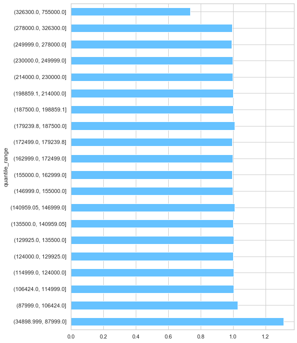
From the above plot, we can see that the model performs relatively well for the middle 18 quantiles. However, the predictions for cheap houses are over-estimated while the predictions for expensive houses are under-estimated. We make corrections to the predictions

# quantile adjustment
q1 = np.quantile(y_pred, 0.1)
q2 = np.quantile(y_pred, 0.90)

q1_factor = 1/1.09
q2_factor = 1/0.95

# Correction
f_q1 = lambda x: x if x > q1 else x * q1_factor
f_q2 = lambda x: x if x < q2 else x * q2_factor

4.6. Predictions

# make predictions on test set
y_test_pred = np.expm1(blend_models_predict(test_normalized))

# correct outliers
corrected_y_test = np.array([f_q1(xi) for xi in y_test_pred])
y_test_pred_series = np.array([f_q2(xi) for xi in corrected_y_test])

submission = pd.read_csv("./data/sample_submission.csv")
submission.iloc[:,1] = np.floor(y_test_pred_series)

submission.to_csv("new_submission.csv", index=False)

Conclusion: This model ranks in the top 5% at the time of the submittal. This is a really good outcome for a relatively simple model without too much feature engineering.