Logistic Regression
This post is part of a three-post series on the topic of Deep Learning. The first part will cover the fundamentals of optimization and more precisely, the logistic regression and its implementation in Python. The second post will cover the basis of layered model. The final post will cover the implementation of a deep neural network.
Table of Content
1. Theory
2. Implementation in Python
3. Data
4. Simple Logistic Regression
5. Conclusion
# load libraries
import numpy as np
import pandas as pd

# personal tools
import TAD_tools

# data generator and data manipulation
from sklearn.datasets import make_classification, make_blobs, make_moons,make_circles
from sklearn.model_selection import train_test_split
from sklearn.metrics import accuracy_score, confusion_matrix

# plotting tools
import matplotlib.pyplot as plt
import seaborn as sns
plt.style.use('ggplot')
%matplotlib inline
1. Theory
The idea behind the logistic regression is to build a linear model (similar to a simple linear regression) in order to predict a binary outcome (0 or 1).
In order to implement a logistic regression, two functions are needed. The first one is a simple linear function (\(L\)) coupled with the sigmoid function (\(\sigma\)). They are defined as:
\[L(x) = b + \sum_{n=1}^{N} w_{n} * x_{n}\]and
\[\sigma(x) = \frac{1}{1+e^{-x}}\]Before we dive deeper into these notions, let’s define a few notations:
- The \(w\)’s are called the weights of the model. The \(b\) is commonly called the bias.
- The input example \(x\) is a n-dimension vector.
The input for our model are defined as:
- A set of \(m\) examples \(\{x_{1},...,x_{m}\}\)
- A set of \(m\) targets \(\{y_{1},...,y_{m}\}\) where \(y_{i}=0\ or\ 1\)
The goal is to find the \(\beta\) of the linear function is order to make the best predictions. A prediction is defined as:
\[a = \sigma(z)\ where\ z=b + \sum_{n=1}^{N} w_{n} * x_{n}\]Indeed the output of the sigmoid function can be interpreted as the probability of the prediction to be either 0 or 1. In order to visualize it, let’s plot the sigmoid function.
# create sigmoid function
z = np.arange(-10,10,0.1)
y = 1 / (1+np.exp(-z))

# plot sigmoid
fig, ax = plt.subplots(figsize=(10,6))

ax.plot(z,y)
ax.set_xlabel('z')
ax.set_ylabel('y')
ax.set_title('Sigmoid function: $\sigma(x)=1/(1+e^{-z})$');
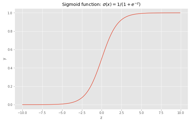
The sigmoid function is defined on the entire range of real numbers and takes values in [0,1]. Therefore, if the output of the linear function is a large value, then the sigmoid will be close to 1 and close to 0 if z is very small. There is one missing aspect to our model. The goal is to predict whether y is equal to 0 or 1, to do so, we will define a threshold.
\[y_{pred}=1\ if\ a\geq0.5\ else\ y_{pred}=0\]Finally, we need to define a performance metric in order to assess how well our model behaves. We call this metric the Loss Function. It represents how close are out predictions to the actual values. The loss function is defined as:
\[L(x)=-log(a)*y-log(1-a)*(1-y)\]# create sigmoid function
x = np.arange(0.00001,0.999999,0.00001)
y_1 = -np.log(x)
y_2 = -np.log(1-x)
# plot sigmoid
fig, ax = plt.subplots(figsize=(10,6))
ax.plot(x,y_1,label="y=1")
ax.plot(x,y_2,label="y=0")
ax.set_xlabel('a')
ax.set_ylabel('y')
ax.set_title('Loss function: $L(x)=-log(a)*y-log(1-a)*(1-y)$')
ax.legend();
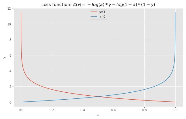
From the above plot, we see that the penalty becomes extremely large is the prediction is incorrect. For instance, if \(y=0\) and \(y_{prob}=0.95\), then the loss is equal to:
-np.log(1-0.95)
2.99573227355399
Whereas if \(y=0\) and \(y_{prob}=0.05\), then the loss is equal to:
-np.log(1-0.05)
0.05129329438755058
Finally, we define the Cost Function as the average of the Loss Function over the entire set of examples.
\[J = \frac{1}{m} \sum_{i=1}^m L(a^{(i)}, y^{(i)})\]The last step of this section consists of the optimization step. Now that the model and the performance metric have been defined, the weights of the model need to be optimized in order to best fit the data. This is where the gradient descent comes into play. The idea behind the optimization is to look at how the performance varies as a function of the weights. To do so, the partial derivatives (slops) of the Cost Function are computed.
\[\frac{\partial J}{\partial w_{i}}\ and\ \frac{\partial J}{\partial b}\]Each parameter is then updated using:
\[\theta_{i} = w_{i} - \alpha*\frac{\partial J}{\partial \theta{i}}\]Where \(\alpha\) is a constant called learning rate.
Based on our definition of the loss, we have:
\[\frac{\partial J}{\partial w} = \frac{1}{m}X(A-Y)^T\] \[\frac{\partial J}{\partial b} = \frac{1}{m} \sum_{i=1}^m (a^{(i)}-y^{(i)})\]Based on the formulas presented above, it is necessary to obtain A (vector of predicted probabilities) in order to obtain the gradients. Therefore, the optimization is before as a two step process:
- Forward propagation: Make predictions using current parameters and compute cost
- Backward propagation: Use predictions to compute gradients and update parameters
2. Implementation in Python
The functions below are used to define the logistic regression model. They are defined as follows:
sigmoid: Simple mathematical function used to apply the sigmoid function to a number or an array.initialize_with_zeros: Creates a vector of zeros of shape (dim, 1) for w and initializes b to 0propagate: Computes the cost function and its gradient for the forward propagationoptimize: Optimizes w and b by running a gradient descent algorithmpredict: Makes a prediction based on a given inputmodel: Builds the logistic regression model
def sigmoid(z):
    """
    Compute the sigmoid of z

    Arguments:
    z -- A scalar or numpy array of any size.

    Return:
    s -- sigmoid(z)
    """

    s = 1 / (1 + np.exp(-z))

    return s
def initialize_with_zeros(dim):
    """
    This function creates a vector of zeros of shape (dim, 1) for w and initializes b to 0.

    Argument:
    dim -- size of the w vector we want (or number of parameters in this case)

    Returns:
    w -- initialized vector of shape (dim, 1)
    b -- initialized scalar (corresponds to the bias)
    """

    w = np.zeros(shape=(dim,1))
    b = 0.0

    assert(w.shape == (dim, 1))
    assert(isinstance(b, float) or isinstance(b, int))

    return w, b
def propagate(w, b, X, Y):
    """
    Computes the cost function and its gradient for the forward propagation

    Arguments:
    w -- weights, a numpy array of size (num_px * num_px * 3, 1)
    b -- bias, a scalar
    X -- data of size (num_px * num_px * 3, number of examples)
    Y -- true "label" vector (containing 0 if non-cat, 1 if cat) of size (1, number of examples)

    Return:
    cost -- negative log-likelihood cost for logistic regression
    dw -- gradient of the loss with respect to w, thus same shape as w
    db -- gradient of the loss with respect to b, thus same shape as b
    """

    m = X.shape[1]                              # number of features

    # FORWARD PROPAGATION (FROM X TO COST)
    A = sigmoid(np.dot(w.T,X)+b)                                    # compute activation SHAPE (1, number of examples)
    cost = (-1/m) * np.sum( Y * np.log(A) + (1-Y) * np.log(1-A) )   # compute cost

    # BACKWARD PROPAGATION (TO FIND GRAD)
    dw = (1/m) * np.dot(X, (A-Y).T)                                 # (m,num) * (1,num).T = (m,1)
    db = (1/m) * (np.sum(A-Y))                                      # (1)

    assert(dw.shape == w.shape)
    assert(db.dtype == float)
    cost = np.squeeze(cost)
    assert(cost.shape == ())

    grads = {"dw": dw,
             "db": db}

    return grads, cost
def optimize(w, b, X, Y, num_iterations, learning_rate, print_cost = False):
    """
    This function optimizes w and b by running a gradient descent algorithm

    Arguments:
    w -- weights, a numpy array of size (num_px * num_px * 3, 1)
    b -- bias, a scalar
    X -- data of shape (num_px * num_px * 3, number of examples)
    Y -- true "label" vector (containing 0 if non-cat, 1 if cat), of shape (1, number of examples)
    num_iterations -- number of iterations of the optimization loop
    learning_rate -- learning rate of the gradient descent update rule
    print_cost -- True to print the loss every 100 steps

    Returns:
    params -- dictionary containing the weights w and bias b
    grads -- dictionary containing the gradients of the weights and bias with respect to the cost function
    costs -- list of all the costs computed during the optimization, this will be used to plot the learning curve.
    """

    costs = []

    for i in range(num_iterations):

        # Cost and gradient calculation (≈ 1-4 lines of code)
        grads, cost = propagate(w, b, X, Y)

        # Retrieve derivatives from grads
        dw = grads["dw"]
        db = grads["db"]

        # update rule (≈ 2 lines of code)
        w = w - learning_rate * dw
        b = b - learning_rate * db

        # Record the costs
        if i % 100 == 0:
            costs.append(cost)

        # Print the cost every 100 training iterations
        if print_cost and i % 100 == 0:
            print ("Cost after iteration %i: %f" %(i, cost))

    params = {"w": w,
              "b": b}

    grads = {"dw": dw,
             "db": db}

    return params, grads, costs
def predict(w, b, X):
    '''
    Predict whether the label is 0 or 1 using learned logistic regression parameters (w, b)

    Arguments:
    w -- weights, a numpy array of size (num_px * num_px * 3, 1)
    b -- bias, a scalar
    X -- data of size (num_px * num_px * 3, number of examples)

    Returns:
    Y_prediction -- a numpy array (vector) containing all predictions (0/1) for the examples in X
    '''

    m = X.shape[1]
    Y_prediction = np.zeros((1,m))
    w = w.reshape(X.shape[0], 1)

    # Compute vector "A" predicting the probabilities of a cat being present in the picture
    A = sigmoid(np.dot(w.T,X)+b)

    for i in range(A.shape[1]):

        # Convert probabilities A[0,i] to actual predictions p[0,i]
        if A[0,i]>0.5:
            Y_prediction[0,i] = 1
        else:
            Y_prediction[0,i] = 0

    assert(Y_prediction.shape == (1, m))

    return Y_prediction
def model(X_train, Y_train, X_test, Y_test, num_iterations = 2000, learning_rate = 0.5, print_cost = False):
    """
    Builds the logistic regression model

    Arguments:
    X_train -- training set represented by a numpy array of shape (num_px * num_px * 3, m_train)
    Y_train -- training labels represented by a numpy array (vector) of shape (1, m_train)
    X_test -- test set represented by a numpy array of shape (num_px * num_px * 3, m_test)
    Y_test -- test labels represented by a numpy array (vector) of shape (1, m_test)
    num_iterations -- hyperparameter representing the number of iterations to optimize the parameters
    learning_rate -- hyperparameter representing the learning rate used in the update rule of optimize()
    print_cost -- Set to true to print the cost every 100 iterations

    Returns:
    d -- dictionary containing information about the model.
    """

    # initialize parameters with zeros (≈ 1 line of code)
    w, b = initialize_with_zeros(X_train.shape[0])

    # Gradient descent (≈ 1 line of code)
    parameters, grads, costs = optimize(w, b, X_train, Y_train, num_iterations, learning_rate, print_cost = print_cost)

    # Retrieve parameters w and b from dictionary "parameters"
    w = parameters["w"]
    b = parameters["b"]

    # Predict test/train set examples (≈ 2 lines of code)
    Y_prediction_test = predict(w, b, X_test)
    Y_prediction_train = predict(w, b, X_train)

    # Print train/test Errors
    print("train accuracy: {:.2f} %".format(100 - np.mean(np.abs(Y_prediction_train - Y_train)) * 100))
    print("test accuracy: {:.2f} %".format(100 - np.mean(np.abs(Y_prediction_test - Y_test)) * 100))

    d = {"costs": costs,
         "Y_prediction_test": Y_prediction_test,
         "Y_prediction_train" : Y_prediction_train,
         "w" : w,
         "b" : b,
         "learning_rate" : learning_rate,
         "num_iterations": num_iterations}

    return d
3. Data
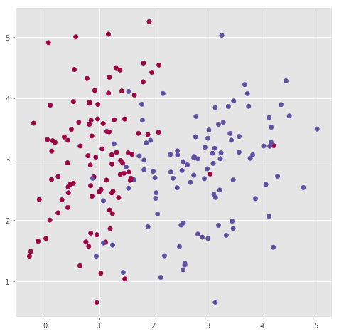
We use sklearn data generator to create a set of inputs (X) with two input features.
# Create data
X, y = make_classification(n_samples=200, n_features=2,
                                            n_informative=2, n_redundant=0,
                                            n_repeated=0, n_classes=2,
                                            n_clusters_per_class=1,
                                            weights=None, flip_y=0.05,
                                            class_sep=0.98, hypercube=True,
                                            shift=2.0, scale=1.0,
                                            shuffle=True, random_state=15)

X_train, X_test, y_train, y_test = train_test_split(X, y, test_size=0.10, random_state=30)

X = X.T
y = y.T
X_train = X_train.T
X_test = X_test.T
y_train = y_train.T.reshape(1,-1)
y_test = y_test.T.reshape(1,-1)
# Visualize the data:
fig, ax = plt.subplots(figsize=(8,8))
plt.scatter(X[0, :], X[1, :], c=y, s=40, cmap=plt.cm.Spectral);
# data shapes
print("X_train: {}".format(X_train.shape))
print("X_test: {}".format(X_test.shape))
print("y_train: {}".format(y_train.shape))
print("y_test: {}".format(y_test.shape))
X_train: (2, 180)
X_test: (2, 20)
y_train: (1, 180)
y_test: (1, 20)
The dataset consists of 200 records (180 are used in the training set). Each record belongs to a class (0 or 1). A logistic regression model is training on the data.
An important step of the analysis consists of understanding the distribution of the data across the various classes. The distribution establish a benchmark accuracy for our model. For instance, if our data is evenly distributed between two classes then our benchmark value (accuracy from a dummy classifier) will be 50%. But if our data was unevenly distributed 90%/10% then the benchmark would be defined as 90%.
# data distribution
unique_elements, counts_elements = np.unique(y, return_counts=True)
print("Frequency of unique values of y:")
print(np.asarray((unique_elements, counts_elements)))

unique_elements, counts_elements = np.unique(y_train, return_counts=True)
print("\nFrequency of unique values of y_train:")
print(np.asarray((unique_elements, counts_elements)))

unique_elements, counts_elements = np.unique(y_test, return_counts=True)
print("\nFrequency of unique values of y_test:")
print(np.asarray((unique_elements, counts_elements)))
Frequency of unique values of y:
[[  0   1]
 [ 99 101]]

Frequency of unique values of y_train:
[[ 0  1]
 [89 91]]

Frequency of unique values of y_test:
[[ 0  1]
 [10 10]]
From the matrices above, the data appears evenly distributed for all sets (full, train, and test).
4. Simple Logistic Regression
d = model(X_train, y_train, X_test, y_test, num_iterations = 2000, learning_rate = 0.5, print_cost = True)
Cost after iteration 0: 0.693147
Cost after iteration 100: 0.287603
Cost after iteration 200: 0.281655
Cost after iteration 300: 0.279128
Cost after iteration 400: 0.277851
Cost after iteration 500: 0.277187
Cost after iteration 600: 0.276836
Cost after iteration 700: 0.276647
Cost after iteration 800: 0.276546
Cost after iteration 900: 0.276490
Cost after iteration 1000: 0.276460
Cost after iteration 1100: 0.276443
Cost after iteration 1200: 0.276434
Cost after iteration 1300: 0.276428
Cost after iteration 1400: 0.276426
Cost after iteration 1500: 0.276424
Cost after iteration 1600: 0.276423
Cost after iteration 1700: 0.276423
Cost after iteration 1800: 0.276422
Cost after iteration 1900: 0.276422
train accuracy: 90.56 %
test accuracy: 95.00 %
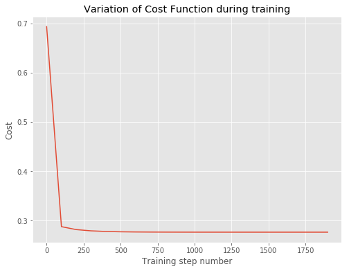
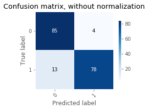
The cost seems to plateau after 1100 iterations. The accuracy on the test set is 95% while the accuracy on the train set is 91%. Overall, the logistic regression performed well on this simple test case.
# Visualize the data:
fig, ax = plt.subplots(figsize=(8,6))
ax.plot(list(range(0,2000,100)), d['costs'])
ax.set_title("Variation of Cost Function during training")
ax.set_xlabel('Training step number')
ax.set_ylabel('Cost');
TAD_tools.plot_confusion_matrix(y_train.T, predict(d['w'], d['b'], X_train).T,
                                classes=np.array([str(x) for x in range(2)]),
                                normalize=False,title=None,cmap=plt.cm.Blues)
print("Accuracy Training = {:.2f}".format(accuracy_score(y_train.T,  predict(d['w'], d['b'], X_train).T)));
Accuracy Training = 0.91
TAD_tools.plot_confusion_matrix(y_test.T, predict(d['w'], d['b'], X_test).T,
                                classes=np.array([str(x) for x in range(2)]),
                                normalize=False,title=None,cmap=plt.cm.Blues)
print("Accuracy Testing = {:.2f}".format(accuracy_score(y_test.T,  predict(d['w'], d['b'], X_test).T)));
Accuracy Testing = 0.95
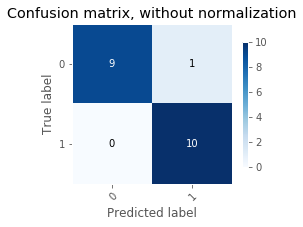
Confusion matrices can be used to identify recurring misclassification. For instance, the logistic regression makes more errors when the true label is 1 than when it is 4. In our example, it does not really matter since the data was randomly generated. However, when working on a real dataset, this pattern can indicate a need for improvement of the model (more data,…).
TAD_tools.plot_decision_boundary_train_test(lambda x: predict(d['w'], d['b'], x.T),
                                            X_train, y_train.T.ravel(),
                                            X_test, y_test.T.ravel())
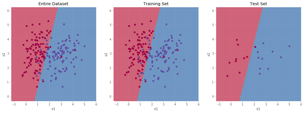
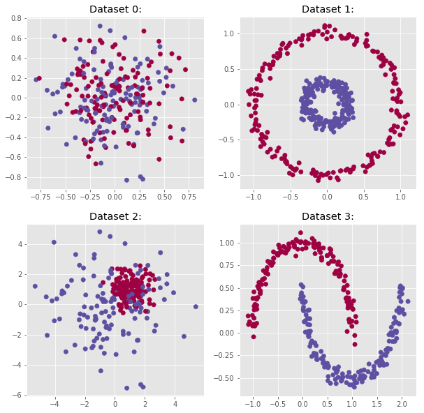
Finally, we now generate a few datasets with complex decision boundaries. The idea is to test the ability of the logistic regression to adapt to more complex situations.
n_samples = 300
outliers_fraction = 0.15
n_outliers = int(outliers_fraction * n_samples)
n_inliers = n_samples - n_outliers
blobs_params = dict(random_state=0, n_samples=n_inliers, n_features=2)
datasets = [
    make_blobs(centers=[[0, 0], [0, 0]], cluster_std=0.3,
               **blobs_params),
    make_circles(n_samples=400, factor=.3, noise=.05, random_state=10),
    make_blobs(centers=[[1, 1], [0, 0]], cluster_std=[0.7, 2.0],
               **blobs_params),
    make_moons(n_samples=n_samples, noise=.05, random_state=0)]
# Visualize the data:
fig, axs = plt.subplots(2, 2, figsize=(10,10))

for row in range(2):
    for col in range(2):
        axs[row,col].scatter(datasets[2*row+col][0][:, 0],
                             datasets[2*row+col][0][:, 1],
                             c=datasets[2*row+col][1],
                             s=40,
                             cmap=plt.cm.Spectral)
        axs[row,col].set_title("Dataset {}:".format(2*row+col));
fig, axs = plt.subplots(2,2,figsize=(10,10))

for i, dataset in enumerate(datasets):
    row = i//2
    col = i%2

    X = dataset[0]
    y = dataset[1]

    X_train, X_test, y_train, y_test = train_test_split(X, y, test_size=0.10, random_state=30)

    X, y = X.T, y.T
    X_train, X_test = X_train.T, X_test.T
    y_train, y_test = y_train.T.reshape(1,-1), y_test.T.reshape(1,-1)

    print("\nDataset {}:".format(i))
    d = model(X_train, y_train, X_test, y_test, num_iterations = 2000, learning_rate = 0.5, print_cost = False)

    TAD_tools.plot_decision_boundary(lambda x: predict(d['w'], d['b'], x.T), X, y, title="Dataset {}:".format(i),ax=axs[row,col])
Dataset 0:
train accuracy: 55.90 %
test accuracy: 30.77 %

Dataset 1:
train accuracy: 31.11 %
test accuracy: 37.50 %

Dataset 2:
train accuracy: 79.04 %
test accuracy: 57.69 %

Dataset 3:
train accuracy: 88.52 %
test accuracy: 86.67 %
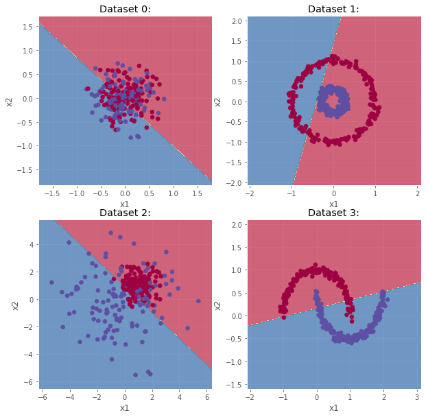
As shown above, when boundaries between classes are not linear, the logistic regression does not perform well (as expected). However, the principle behind linear classification can be used and combined in order to make more complex model. A new type of model combining the efficiency of the logistic regression and a non-linear aspect is the natural next step towards deep learning.
5. Conclusion
Pros
- Simple to implement.
- Few hyperparameters.
- Easy to interpret and visualize (up to three dimensions).
- Works for both binary and multi-class classification.
- Can be upgraded with regularization (Ridge or Lasso)
Cons
- Works well if data relationships are linear.
- Too simple to capture complex relationships.
In conclusion, a logistic regression can be seen as the first step of the path to a more complex model. It is often use as a mean to assess the complexity of a problem and obtain quick and rough results.
In part of this series, we will cover the basic of deep learning and how we can leverage the basics of the logistic regression to implement more complex models.