Neural Network
This notebook covers the basics of neural networks and their implementation in Python. In Part 1 of this series, we went over the logistic regression and concluded with mixed feelings. Indeed, the logistic regression appeared to be a simple yet effective model with important limitations. In this new post, we will see how we can leverage the theory behind logistic regression to build a model with improved predictive power. These is where Neural Networks come into play.
Neural Networks were created in an intent to mimic the human vision and the brain structure. Instead of having the entire information process by a neuron, it is process by an network of neurons. Each neuron serves a basic function (detect curves, detect straight lines…) then the information is conveyed to another layer in charge of detecting more complex patter.
Table of Content
1. Notation
2. Theory
3. Implementation in Python
4. Data
5. Simple Neural Network
6. Effect of the Hidden Layer Size
7. Conclusion
# load libraries
import numpy as np
import pandas as pd

# personal tools
import TAD_tools_v00

# data generator and data manipulation
from sklearn.datasets import make_classification, make_blobs, make_moons, make_circles, make_classification
from sklearn.model_selection import train_test_split
from sklearn.metrics import accuracy_score, confusion_matrix

# plotting tools
import matplotlib.pyplot as plt
import seaborn as sns
plt.style.use('ggplot')
%matplotlib inline
1. Notations
The following notations are used in this notebook:
- \(m\) is the number of feature of the input
- Type: integer
- \(n\) is the number of input examples
- Type: integer
- \(x\) is the set of input data
- Type: Array
- Size: \((m*n)\)
- Components: \(x^{(i)}\) of size \((m*1)\)
- \(n^{[1]}\) is the number of neurons in the hidden layer
- Type: integer
- \(W^{[1]}\) are the weights of the layer 1 (hidden)
- Type: Array
- Size: \((n^{[1]}*m)\)
- \(W^{[2]}\) are the weights of the layer 2 (output)
- Type: Array
- Size: \((1*n^{[1]})\)
- \(b^{[l]}\) are the bias of the layer 1 (hidden)
- Type: Array
- Size: \((n^{[1]}*1)\)
- \(b^{[2]}\) are the bias of the layer 2 (output)
- Type: Array
- Size: \((1*1)\)
- \(a^{[1]}\) is the output of the first layer
- Type: Array
- Size: \((n^{[1]}*n)\)
- Components: \(a^{[1] (i)}\)
2. Theory
2.1. Components
The simple neural network model is made of the following components:
- The input layer (i.e. the input data)
- One hidden layer
- One output layer
The hidden layer is made of an ensemble of neurons each equipped with the following two tools:
- A set of weights \(\{w_{1},..,w_{m}\}\) and a bias term \(b\).
- An activation function which adds a non-linear behavior to its neuron.
2.2. Architecture
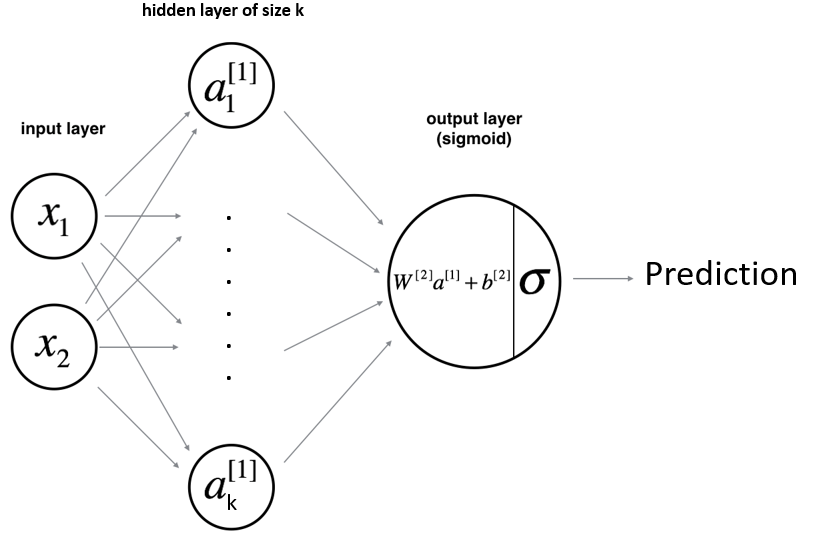
As shown above, the input vector \(X=\{x_{1},x_{2}\}\) passes through the first hidden layer. The output of the hidden layer are then used as an input for the output layer. Finally, the output of the last layer is used to make a prediction.
Let’s take an example where the hidden layer is made of 2 hidden units. The equations of the model are:
\(a_{1}^{[1]}=g(w_{1,1}^{[1]}*x_{1}+w_{1,2}^{[1]}*x_{2}+b_{1}^{[1]})\)
\(a_{2}^{[1]}=g(w_{2,1}^{[1]}*x_{1}+w_{2,2}^{[1]}*x_{2}+b_{2}^{[1]})\)
Then:
\(y_{prob}=\sigma(w_{1}^{[2]}*a_{1}^{[1]}+w_{2}^{[2]}*a_{2}^{[1]}+b^{[2]})\)
2.3. Activation Functions
The activation of the output layer is the sigmoid. This choice is based on the nature of the output, the output layer gives a probability (between 0 and 1). However, the activation layer of the hidden units can be chosen amongst a larger set of functions:
- tanh
- ReLU (Rectified Linear Unit)
- Leaky RelU
- Step
- Linear
# Define the range for plot
x = np.linspace(-2,2,100)

# Define activation functions over range
f_tanh = np.tanh(x)
f_relu = np.maximum(x,0)
f_leaky_relu = np.maximum(x,0.01*x)
f_step = x / 2 / np.abs(x) + 1/2
f_linear = x
# Plot activation functions
fig, axs = plt.subplots(1,2,figsize=(16,6))
axs[0].plot(x, f_tanh, label='tanh', linestyle='-.')
axs[0].plot(x, f_step, label='step')
axs[0].plot(x, f_linear, label='linear', color='orchid', linestyle='--')
axs[1].plot(x, f_relu, label='ReLU: max(x, 0)')
axs[1].plot(x, f_leaky_relu, label='Leaky ReLU: max(x, 0.01*x)', linestyle='--')
axs[0].legend()
axs[1].legend()
fig.suptitle('Activation Functions');
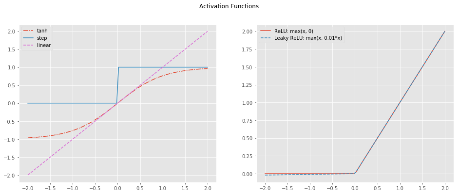
NOTE: For the rest of this post, the tanh function is used. It performs relatively well as it creates the non-linearity needed while spanning between -1 and 1. Small values helps with the optimization.
2.4. Cost Function
Finally, we define the Cost Function as the average of the Loss Function over the entire set of examples.
\[J = \frac{1}{m} \sum_{i=1}^m L(a^{(i)}, y^{(i)})\]2.5. Optimization
Similarly to the logistic regression, a gradient descent is performed to optimize the various weights of the network. The optimization is performed as a three-step process:
- Forward propagation: Compute the predictions and the various outputs of each layer.
- Backward propagation: Use the results from the previous step to compute the partial derivative of the cost function with respect to each weight.
- Update the weights
Below are the formulas used to compute the gradients.
\(\frac{\partial J }{ \partial z_{2}^{(i)} } = \frac{1}{m} (a^{[2](i)} - y^{(i)})\)
\(\frac{\partial J }{ \partial W_2 } = \frac{\partial J }{ \partial z_{2}^{(i)} } a^{[1] (i) T}\)
\(\frac{\partial J }{ \partial b_2 } = \sum_i{\frac{\partial J }{ \partial z_{2}^{(i)}}}\)
\(\frac{\partial J }{ \partial z_{1}^{(i)} } = W_2^T \frac{\partial J }{ \partial z_{2}^{(i)} } * ( 1 - a^{[1] (i) 2})\)
\(\frac{\partial J }{ \partial W_1 } = \frac{\partial J }{ \partial z_{1}^{(i)} } X^T\)
\(\frac{\partial J _i }{ \partial b_1 } = \sum_i{\frac{\partial J }{ \partial z_{1}^{(i)}}}\)
- Note that \(*\) denotes element-wise multiplication.
- The notation you will use is common in deep learning coding:
- dW1 = \(\frac{\partial J }{ \partial W_1 }\)
- db1 = \(\frac{\partial J }{ \partial b_1 }\)
- dW2 = \(\frac{\partial J }{ \partial W_2 }\)
- db2 = \(\frac{\partial J }{ \partial b_2 }\)
3. Implementation in Python
The functions below are used to define the neural network model. They are defined as follows:
layer_sizes: Establish the architecture of the modelinitialize_parameters: Initialize the weight matricesforward_propagation: Forward propagationcompute_cost: Compute binary cross-entropybackward_propagation: Compute gradientsupdate_parameters: Update weights based on computed gradientsnn_model: Builds the neural network modelpredict: Make prediction using the trained model
def layer_sizes(X, Y, n_h):
    """
    Arguments:
    X -- input dataset of shape (input size, number of examples)
    Y -- labels of shape (output size, number of examples)
    n_h -- number of hidden units

    Returns:
    n_x -- the size of the input layer
    n_h -- the size of the hidden layer
    n_y -- the size of the output layer
    """

    n_x = X.shape[0]
    n_y = Y.shape[0]

    return (n_x, n_h, n_y)
def initialize_parameters(n_x, n_h, n_y):
    """
    Argument:
    n_x -- size of the input layer
    n_h -- size of the hidden layer
    n_y -- size of the output layer

    Returns:
    params -- python dictionary containing your parameters:
                    W1 -- weight matrix of shape (n_h, n_x)
                    b1 -- bias vector of shape (n_h, 1)
                    W2 -- weight matrix of shape (n_y, n_h)
                    b2 -- bias vector of shape (n_y, 1)
    """

    # set random seed
    np.random.seed(2)

    # hidden layer
    W1 = np.random.randn(n_h, n_x) * 0.01
    b1 = np.zeros((n_h, 1))

    # output layer
    W2 = np.random.randn(n_y, n_h) * 0.01
    b2 = np.zeros((n_y, 1))

    # store results
    paramters = {'W1':W1,
                 'b1':b1,
                 'W2':W2,
                 'b2':b2}

    return paramters
def forward_propagation(X, parameters):
    """
    Argument:
    X -- input data of size (n_x, m)
    parameters -- python dictionary containing your parameters (output of initialization function)

    Returns:
    A2 -- The sigmoid output of the second activation
    cache -- a dictionary containing "Z1", "A1", "Z2" and "A2"
    """
    # retrieve parameters
    W1 = parameters['W1']   # hidden layer
    b1 = parameters['b1']   # hidden layer
    W2 = parameters['W2']   # output layer
    b2 = parameters['b2']   # output layer

    # Implement Forward Propagation to calculate A2 (probabilities)
    Z1 = np.dot(W1, X) + b1
    A1 = np.tanh(Z1)
    Z2 = np.dot(W2, A1) + b2
    A2 = TAD_tools_v00.sigmoid(Z2)

    assert(A2.shape == (1, X.shape[1]))

    cache = {"Z1": Z1,
             "A1": A1,
             "Z2": Z2,
             "A2": A2}

    return A2, cache
def compute_cost(A2, Y, parameters):
    """
    Computes the cross-entropy cost given in equation (13)

    Arguments:
    A2 -- The sigmoid output of the second activation, of shape (1, number of examples)
    Y -- "true" labels vector of shape (1, number of examples)
    parameters -- python dictionary containing your parameters W1, b1, W2 and b2

    Returns:
    cost -- cross-entropy cost given equation (13)
    """

    # number of training examples
    m = Y.shape[1]

    # compute cost and squeeze to single float
    cost = -1 / m * np.sum(np.multiply(np.log(A2),Y) + np.multiply(np.log(1 - A2),1 - Y))
    cost = np.squeeze(cost)

    return cost
def backward_propagation(parameters, cache, X, Y):
    """
    Implement the backward propagation using the instructions above.

    Arguments:
    parameters -- python dictionary containing our parameters
    cache -- a dictionary containing "Z1", "A1", "Z2" and "A2".
    X -- input data of shape (2, number of examples)
    Y -- "true" labels vector of shape (1, number of examples)

    Returns:
    grads -- python dictionary containing your gradients with respect to different parameters
    """

    # number of training examples
    m = Y.shape[1]

    # retrieve parameters
    W1 = parameters['W1']   # hidden layer
    b1 = parameters['b1']   # hidden layer
    W2 = parameters['W2']   # output layer
    b2 = parameters['b2']   # output layer

    # retrieve cache
    Z1 = cache['Z1']
    A1 = cache['A1']
    Z2 = cache['Z2']
    A2 = cache['A2']

    # compute gradients from output layer
    dZ2 = A2 - Y
    dW2 = np.dot(dZ2, A1.T) * (1/m)
    db2 = np.sum(dZ2, axis=1, keepdims=True) * (1/m)

    # compute gradients from hidden layer
    dZ1 = np.dot(W2.T, dZ2) * (1 - np.power(A1, 2))
    dW1 = np.dot(dZ1, X.T) * (1/m)
    db1 = np.sum(dZ1, axis=1, keepdims=True) * (1/m)

    # store results
    grads = {"dW1": dW1,
             "db1": db1,
             "dW2": dW2,
             "db2": db2}

    return grads
def update_parameters(parameters, grads, learning_rate = 1.2):
    """
    Updates parameters using the gradient descent update rule given above

    Arguments:
    parameters -- python dictionary containing your parameters
    grads -- python dictionary containing your gradients

    Returns:
    parameters -- python dictionary containing your updated parameters
    """

    # retrieve parameters
    W1 = parameters['W1']     # hidden layer
    b1 = parameters['b1']     # hidden layer
    W2 = parameters['W2']     # output layer
    b2 = parameters['b2']     # output layer

    # retrieve gradients
    dW1 = grads['dW1']        # hidden layer
    db1 = grads['db1']        # hidden layer
    dW2 = grads['dW2']        # output layer
    db2 = grads['db2']        # output layer

    # update parameters
    W1 -= learning_rate * dW1   # hidden layer
    b1 -= learning_rate * db1   # hidden layer
    W2 -= learning_rate * dW2   # output layer
    b2 -= learning_rate * db2   # output layer

    # store parameters
    parameters = {'W1':W1,
                 'b1':b1,
                 'W2':W2,
                 'b2':b2}

    return parameters
def nn_model(X, Y, n_h, num_iterations = 10000, print_cost=False):
    """
    Arguments:
    X -- dataset of shape (2, number of examples)
    Y -- labels of shape (1, number of examples)
    n_h -- size of the hidden layer
    num_iterations -- Number of iterations in gradient descent loop
    print_cost -- if True, print the cost every 1000 iterations

    Returns:
    parameters -- parameters learned by the model. They can then be used to predict.
    """
    # set random seed for parameter initialization
    np.random.seed(3)

    # extract number of features from input data and dimension of prediction (1)
    n_x = layer_sizes(X, Y, n_h)[0]
    n_y = layer_sizes(X, Y, n_h)[2]

    # store costs and step count
    iteration_steps = []
    cost_steps = []

    # initialize parameters
    parameters = initialize_parameters(n_x, n_h, n_y)

    # retrieve initialized parameters
    W1 = parameters['W1']   # hidden layer
    b1 = parameters['b1']   # hidden layer
    W2 = parameters['W2']   # output layer
    b2 = parameters['b2']   # output layer

    # Forward > Backward > Parameter update
    for i in range(0, num_iterations):

        # forward propagation
        A2, cache = forward_propagation(X, parameters)

        # compute cost
        cost = compute_cost(A2, Y, parameters)

        # backward propagation
        grads = backward_propagation(parameters, cache, X, Y)

        # update parameters - gradient descent
        parameters = update_parameters(parameters, grads, learning_rate = 1.2)

        # print the cost every 1000 iterations
        iteration_steps.append(i)
        cost_steps.append(cost)
        if print_cost and i % 1000 == 0:
            print ("Cost after iteration %i: %f" %(i, cost))

    # print termination and final accuracy
    y_proba, _ = forward_propagation(X, parameters)
    y_pred = y_proba > 0.5
    accuracy = np.sum(y_pred==y) / y.shape[1]
    print("Training: DONE....")
    print('Train Accuracy: {0:.2%}'.format(accuracy))

    return parameters, iteration_steps, cost_steps
def predict(parameters, X):
    """
    Using the learned parameters, predicts a class for each example in X

    Arguments:
    parameters -- python dictionary containing your parameters
    X -- input data of size (n_x, m)

    Returns
    predictions -- vector of predictions of our model (red: 0 / blue: 1)
    """

    A2, cache = forward_propagation(X, parameters)
    predictions = A2 > 0.5

    return predictions
4. Data
Let’s first test the model against the four datasets generated at the end of the Part 1 post.
# number of data-points
n_samples = 300
outliers_fraction = 0.15
n_outliers = int(outliers_fraction * n_samples)
n_inliers = n_samples - n_outliers
blobs_params = dict(random_state=0, n_samples=n_inliers, n_features=2)
datasets = [
    make_blobs(centers=[[0, 0], [0, 0]], cluster_std=0.3,
               **blobs_params),
    make_circles(n_samples=400, factor=.3, noise=.05, random_state=10),
    make_blobs(centers=[[1, 1], [0, 0]], cluster_std=[0.7, 2.0],
               **blobs_params),
    make_moons(n_samples=n_samples, noise=.05, random_state=0)]
# Visualize the data:
fig, axs = plt.subplots(2, 2, figsize=(10,10))

for row in range(2):
    for col in range(2):
        axs[row,col].scatter(datasets[2*row+col][0][:, 0],
                             datasets[2*row+col][0][:, 1],
                             c=datasets[2*row+col][1],
                             s=40,
                             cmap=plt.cm.Spectral)
        axs[row,col].set_title("Dataset {}:".format(2*row+col));
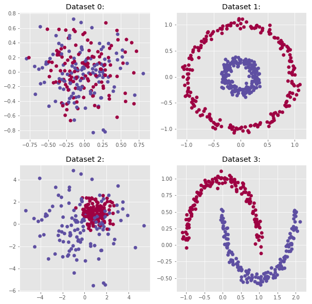
From the plots shown above, one can expect the model to perfectly predict the classes for Dataset 1 and 3. Indeed, the class distributions for the datasets 0 and 2 are not clearly defined.
5. Simple Neural Network
# Tool function
def plot_decision_boundary(model, X, y, title=None, ax=None):
    import matplotlib.pyplot as plt
    # Set min and max values and give it some padding
    x_min, x_max = X[0, :].min() - 1, X[0, :].max() + 1
    y_min, y_max = X[1, :].min() - 1, X[1, :].max() + 1

    h = 0.01

    # Generate a grid of points with distance h between them
    xx, yy = np.meshgrid(np.arange(x_min, x_max, h), np.arange(y_min, y_max, h))

    # Predict the function value for the whole grid
    Z = model(np.c_[xx.ravel(), yy.ravel()].T)
    Z = Z.reshape(xx.shape)

    # Plot the contour and training examples
    if ax is None:
        fig, ax = plt.subplots(figsize=(8,8))
    ax.contourf(xx, yy, Z, cmap=plt.cm.Spectral, alpha=0.7)
    ax.set_ylabel('x2')
    ax.set_xlabel('x1')
    ax.scatter(X[0, :], X[1, :], c=y.ravel().T, cmap=plt.cm.Spectral)
    ax.set_title(title);
5.1: Dataset 0
# extract data-points
X = datasets[0][0].T
y = datasets[0][1].reshape(1,-1)

# print shapes
print("X shape:{}".format(X.shape))
print("y shape:{}".format(y.shape))
X shape:(2, 255)
y shape:(1, 255)
# set number of hidden units
n_h = 4

# build and train model
parameters, iteration_steps, cost_steps = nn_model(X, y, n_h, num_iterations = 10000, print_cost=False)
Training: DONE....
Train Accuracy: 56.08%
# plot both the decision boundary and the cost function
fig, axs = plt.subplots(1, 2, figsize=(16,8))
plot_decision_boundary(lambda x: predict(parameters, x), X, y, title=None, ax=axs[0])
axs[1].plot(iteration_steps,cost_steps)
axs[1].set_xlabel('Iteration Number')
axs[1].set_ylabel('Cost function')
axs[0].set_title('Decision Boundary')
axs[1].set_title('Cost Function during training');
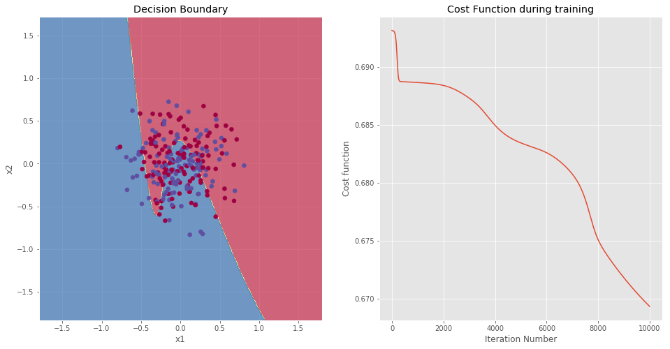
NOTE: The accuracy on the training set is 56.08%. Such a low value was expected based on the data distribution. The two data clusters appear to be fused into a single cluster. Therefore, the model performs slightly better than a random guess (50% accuracy). In is interesting to note the shape of the decision boundary. The greater complexity of the model leads to more complex decision boundary.
5.2: Dataset 1
# extract data-points
X = datasets[1][0].T
y = datasets[1][1].reshape(1,-1)

# print shapes
print("X shape:{}".format(X.shape))
print("y shape:{}".format(y.shape))
X shape:(2, 400)
y shape:(1, 400)
# set number of hidden units
n_h = 4

# build and train model
parameters, iteration_steps, cost_steps = nn_model(X, y, n_h, num_iterations = 10000, print_cost=False)
Training: DONE....
Train Accuracy: 100.00%
# plot both the decision boundary and the cost function
fig, axs = plt.subplots(1, 2, figsize=(16,8))
plot_decision_boundary(lambda x: predict(parameters, x), X, y, title=None, ax=axs[0])
axs[1].plot(iteration_steps,cost_steps)
axs[1].set_xlabel('Iteration Number')
axs[1].set_ylabel('Cost function')
axs[0].set_title('Decision Boundary')
axs[1].set_title('Cost Function during training');
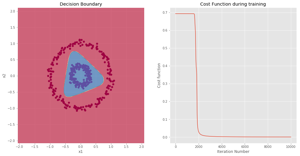
NOTE: As expected, the model is able to perfectly classify each data-point.
5.3: Dataset 2
# extract data-points
X = datasets[2][0].T
y = datasets[2][1].reshape(1,-1)

# print shapes
print("X shape:{}".format(X.shape))
print("y shape:{}".format(y.shape))
X shape:(2, 255)
y shape:(1, 255)
# set number of hidden units
n_h = 4

# build and train model
parameters, iteration_steps, cost_steps = nn_model(X, y, n_h, num_iterations = 10000, print_cost=False)
Training: DONE....
Train Accuracy: 87.06%
# plot both the decision boundary and the cost function
fig, axs = plt.subplots(1, 2, figsize=(16,8))
plot_decision_boundary(lambda x: predict(parameters, x), X, y, title=None, ax=axs[0])
axs[1].plot(iteration_steps,cost_steps)
axs[1].set_xlabel('Iteration Number')
axs[1].set_ylabel('Cost function')
axs[0].set_title('Decision Boundary')
axs[1].set_title('Cost Function during training');
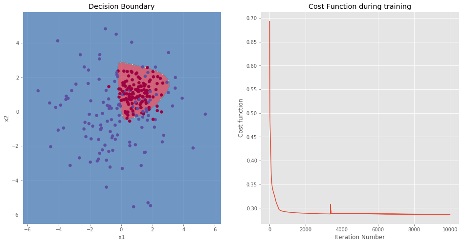
NOTE: This example is the most interesting of the four datasets. Indeed, the data clusters are not perfectly separated. However, by looking at the data, one can define a perimeter which envelopes the red cluster. After running the model, the training accuracy is 87.06%, this is a good improvement over the predictions of the logistic regression.
5.4: Dataset 3
# extract data-points
X = datasets[3][0].T
y = datasets[3][1].reshape(1,-1)

# print shapes
print("X shape:{}".format(X.shape))
print("y shape:{}".format(y.shape))
X shape:(2, 300)
y shape:(1, 300)
# set number of hidden units
n_h = 4

# build and train model
parameters, iteration_steps, cost_steps = nn_model(X, y, n_h, num_iterations = 10000, print_cost=False)
Training: DONE....
Train Accuracy: 100.00%
# plot both the decision boundary and the cost function
fig, axs = plt.subplots(1, 2, figsize=(16,8))
plot_decision_boundary(lambda x: predict(parameters, x), X, y, title=None, ax=axs[0])
axs[1].plot(iteration_steps,cost_steps)
axs[1].set_xlabel('Iteration Number')
axs[1].set_ylabel('Cost function')
axs[0].set_title('Decision Boundary')
axs[1].set_title('Cost Function during training');
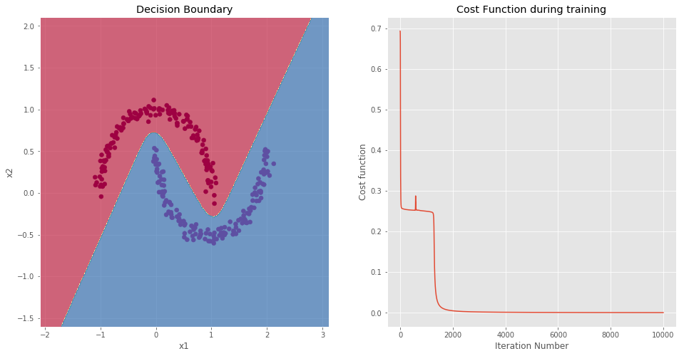
NOTE: As expected, the model is able to perfectly classify each data-point.
6. Effect of the Hidden Layer Size
The model used to make predictions using four examples treated in Section 5 had a hidden layer equipped with four hidden units. In order to understand how this hyper-parameter can be chosen, we compute the accuracy of the predictions on dataset 2.
# extract data-points
X = datasets[2][0].T
y = datasets[2][1].reshape(1,-1)
n_h_list = [1,2,3,4,5,10,15,20]

fig, axs = plt.subplots(4, 2, figsize=(16,32))

for i, n_h in enumerate(n_h_list):
    row = i // 2
    col = i % 2

    # build and train model
    parameters, iteration_steps, cost_steps = nn_model(X, y, n_h, num_iterations = 10000, print_cost=False)

    # plot the cost function
    plot_decision_boundary(lambda x: predict(parameters, x), X, y, title=None, ax=axs[row,col])
    axs[row,col].set_title('{} hidden units'.format(n_h))
Training: DONE....
Train Accuracy: 79.22%
Training: DONE....
Train Accuracy: 85.49%
Training: DONE....
Train Accuracy: 85.49%
Training: DONE....
Train Accuracy: 87.06%
Training: DONE....
Train Accuracy: 87.84%
Training: DONE....
Train Accuracy: 90.59%
Training: DONE....
Train Accuracy: 90.59%
Training: DONE....
Train Accuracy: 90.59%
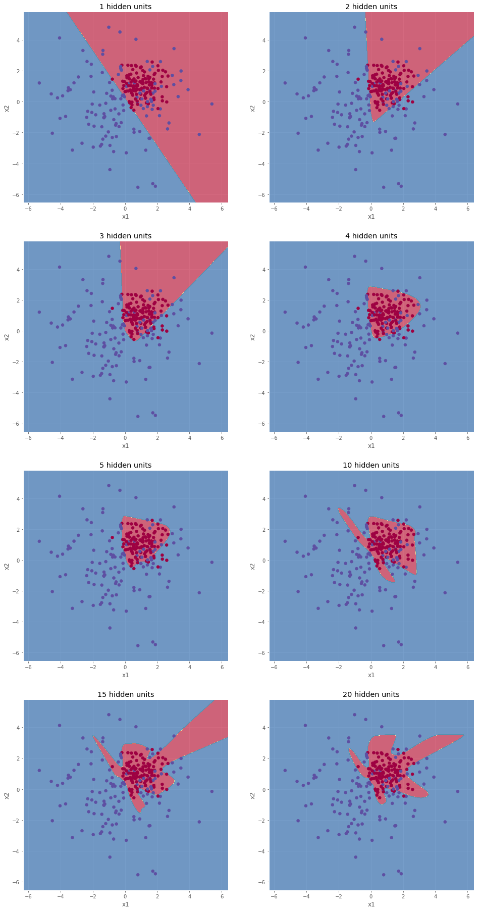
As shown above, the decision boundary becomes more and more complex as the number of hidden units increases. The results obtained with 10, 15, and 20 hidden units are considered as over-fitted. Indeed, the models try to much to envelope each data points (even the isolated ones). In order to obtain a good generalized model, over-fitted needs to be avoided. For this reason, the model obtained with 5 hidden units is the preferred one. Note that to fully evaluate the models, it is necessary to test the prediction power on unseen data (the test set).
7. Conclusion
In conclusion, the addition of the hidden layer to our simple logistic regression model lead to great improvements. This second step toward a complete Deep Neural Network laid the basis for a layered model.
Pros
- Better than simple logistic regression.
- Relatively fast to train.
- Easy to interpret and visualize (up to three dimensions).
- Works for both binary and multi-class classification.
- Can be upgraded with regularization (Ridge or Lasso) and/or mini-batch gradient descent.
Cons
- Requires tuning of the new hyper-parameters (number of hidden units and activation functions)
- Prone to over fitting without proper tuning.