Predict Future Sales

Final project for “How to win a data science competition” Coursera course
Table of Contents
Introduction
This challenge serves as final project for the “How to win a data science competition” Coursera course.
In this competition you will work with a challenging time-series dataset consisting of daily sales data, kindly provided by one of the largest Russian software firms - 1C Company.
We are asking you to predict total sales for every product and store in the next month. By solving this competition you will be able to apply and enhance your data science skills.
The full project description and dataset can be found here.
Data and Competition
Data Structure
We are provided with daily historical sales data. The task is to forecast the total amount of products sold in every shop for the test set. Note that the list of shops and products slightly changes every month. Creating a robust model that can handle such situations is part of the challenge.
File descriptions
sales_train.csv- the training set. Daily historical data from January 2013 to October 2015.test.csv- the test set. You need to forecast the sales for these shops and products for November 2015.sample_submission.csv- a sample submission file in the correct format.items.csv - supplementalinformation about the items/products.item_categories.csv- supplemental information about the items categories.shops.csv- supplemental information about the shops.
Data fields
ID- an Id that represents a (Shop, Item) tuple within the test setshop_id- unique identifier of a shopitem_id- unique identifier of a productitem_category_id- unique identifier of item categoryitem_cnt_day- number of products sold. You are predicting a monthly amount of this measureitem_price- current price of an itemdate - datein format dd/mm/yyyydate_block_num- a consecutive month number, used for convenience. January 2013 is 0, February 2013 is 1,…, October 2015 is 33item_name- name of itemshop_name- name of shopitem_category_name- name of item category
Objective
The goal of this competition is to predict the total amount of products sold in every shop for the test set. The list of shops and products changes each month. Submissions are evaluated by root mean squared error (RMSE). True target values are clipped into [0,20] range.
Load Libraries and Dataset
import numpy as np
import pandas as pd

import matplotlib.pyplot as plt
import seaborn as sns
plt.style.use('ggplot')

from tqdm import tqdm_notebook
from ipywidgets import IntProgress

import pickle
from itertools import product
import gc
import time

from sklearn.preprocessing import MinMaxScaler, LabelEncoder

from sklearn.preprocessing import LabelEncoder
from sklearn.feature_selection import SelectFromModel
from sklearn.model_selection import train_test_split, cross_val_score, KFold
from sklearn.linear_model import ElasticNet, Lasso, Ridge, RidgeCV, LassoCV, ElasticNetCV, BayesianRidge, LinearRegression
from sklearn.tree import DecisionTreeRegressor, ExtraTreeClassifier
from sklearn.svm import SVR
from sklearn.ensemble import RandomForestRegressor,  GradientBoostingRegressor, ExtraTreesRegressor
from sklearn.neighbors import KNeighborsRegressor
from sklearn.model_selection import GridSearchCV, ShuffleSplit
from sklearn.preprocessing import RobustScaler
from sklearn.pipeline import make_pipeline
from sklearn.metrics import mean_squared_error

from lightgbm import LGBMRegressor
import lightgbm as lgb
import xgboost as xgb
from xgboost import XGBRegressor

np.random.seed(42)
We load each csv file in an independent Padas DataFrame.
sales_train = pd.read_csv('./competitive-data-science-predict-future-sales/sales_train.csv', parse_dates=['date'])
sales_test = pd.read_csv('./competitive-data-science-predict-future-sales/test.csv')
sample_submission = pd.read_csv('./competitive-data-science-predict-future-sales/sample_submission.csv')
items = pd.read_csv('./competitive-data-science-predict-future-sales/items.csv')
item_categories = pd.read_csv('./competitive-data-science-predict-future-sales/item_categories.csv')
shops = pd.read_csv('./competitive-data-science-predict-future-sales/shops.csv')
sample_submission.head(3)
| ID | item_cnt_month | |
|---|---|---|
| 0 | 0 | 0.5 |
| 1 | 1 | 0.5 |
| 2 | 2 | 0.5 |
Let’s explore the datasets by first looking at:
- The dataset shapes
- The dataset columns
- The data info
Sales Dataset
print("Sales Train")
sales_train.head()
Sales Train
| date | date_block_num | shop_id | item_id | item_price | item_cnt_day | |
|---|---|---|---|---|---|---|
| 0 | 2013-02-01 | 0 | 59 | 22154 | 999.00 | 1.0 |
| 1 | 2013-03-01 | 0 | 25 | 2552 | 899.00 | 1.0 |
| 2 | 2013-05-01 | 0 | 25 | 2552 | 899.00 | -1.0 |
| 3 | 2013-06-01 | 0 | 25 | 2554 | 1709.05 | 1.0 |
| 4 | 2013-01-15 | 0 | 25 | 2555 | 1099.00 | 1.0 |
The item_cnt_dat colum contains positive values for sales and negative values for returns.
print("Sales Train set shape", sales_train.shape)
Sales Train set shape (2935849, 6)
sales_train.info()
<class 'pandas.core.frame.DataFrame'>
RangeIndex: 2935849 entries, 0 to 2935848
Data columns (total 6 columns):
date              datetime64[ns]
date_block_num    int64
shop_id           int64
item_id           int64
item_price        float64
item_cnt_day      float64
dtypes: datetime64[ns](1), float64(2), int64(3)
memory usage: 134.4 MB
print("Null records")
sales_train.isnull().sum()
Null records
date              0
date_block_num    0
shop_id           0
item_id           0
item_price        0
item_cnt_day      0
dtype: int64
print('Description')
sales_train.describe()
Description
| date_block_num | shop_id | item_id | item_price | item_cnt_day | |
|---|---|---|---|---|---|
| count | 2.935849e+06 | 2.935849e+06 | 2.935849e+06 | 2.935849e+06 | 2.935849e+06 |
| mean | 1.456991e+01 | 3.300173e+01 | 1.019723e+04 | 8.908532e+02 | 1.242641e+00 |
| std | 9.422988e+00 | 1.622697e+01 | 6.324297e+03 | 1.729800e+03 | 2.618834e+00 |
| min | 0.000000e+00 | 0.000000e+00 | 0.000000e+00 | -1.000000e+00 | -2.200000e+01 |
| 25% | 7.000000e+00 | 2.200000e+01 | 4.476000e+03 | 2.490000e+02 | 1.000000e+00 |
| 50% | 1.400000e+01 | 3.100000e+01 | 9.343000e+03 | 3.990000e+02 | 1.000000e+00 |
| 75% | 2.300000e+01 | 4.700000e+01 | 1.568400e+04 | 9.990000e+02 | 1.000000e+00 |
| max | 3.300000e+01 | 5.900000e+01 | 2.216900e+04 | 3.079800e+05 | 2.169000e+03 |
print("Sales Test")
sales_test.head()
Sales Test
| ID | shop_id | item_id | |
|---|---|---|---|
| 0 | 0 | 5 | 5037 |
| 1 | 1 | 5 | 5320 |
| 2 | 2 | 5 | 5233 |
| 3 | 3 | 5 | 5232 |
| 4 | 4 | 5 | 5268 |
print("Sales Test set shape", sales_test.shape)
Sales Test set shape (214200, 3)
sales_test.info()
<class 'pandas.core.frame.DataFrame'>
RangeIndex: 214200 entries, 0 to 214199
Data columns (total 3 columns):
ID         214200 non-null int64
shop_id    214200 non-null int64
item_id    214200 non-null int64
dtypes: int64(3)
memory usage: 4.9 MB
Item Dataset
print("Items")
items.head()
Items
| item_name | item_id | item_category_id | |
|---|---|---|---|
| 0 | ! ВО ВЛАСТИ НАВАЖДЕНИЯ (ПЛАСТ.) D | 0 | 40 |
| 1 | !ABBYY FineReader 12 Professional Edition Full... | 1 | 76 |
| 2 | ***В ЛУЧАХ СЛАВЫ (UNV) D | 2 | 40 |
| 3 | ***ГОЛУБАЯ ВОЛНА (Univ) D | 3 | 40 |
| 4 | ***КОРОБКА (СТЕКЛО) D | 4 | 40 |
print("Items shape", items.shape)
Items shape (22170, 3)
print("Null records")
items.isnull().sum()
Null records
item_name           0
item_id             0
item_category_id    0
dtype: int64
items.info()
<class 'pandas.core.frame.DataFrame'>
RangeIndex: 22170 entries, 0 to 22169
Data columns (total 3 columns):
item_name           22170 non-null object
item_id             22170 non-null int64
item_category_id    22170 non-null int64
dtypes: int64(2), object(1)
memory usage: 519.7+ KB
Item Categories Dataset
print("Item Categories")
item_categories.head()
Item Categories
| item_category_name | item_category_id | |
|---|---|---|
| 0 | PC - Гарнитуры/Наушники | 0 |
| 1 | Аксессуары - PS2 | 1 |
| 2 | Аксессуары - PS3 | 2 |
| 3 | Аксессуары - PS4 | 3 |
| 4 | Аксессуары - PSP | 4 |
print("Item categories shape", item_categories.shape)
Item categories shape (84, 2)
item_categories.info()
<class 'pandas.core.frame.DataFrame'>
RangeIndex: 84 entries, 0 to 83
Data columns (total 2 columns):
item_category_name    84 non-null object
item_category_id      84 non-null int64
dtypes: int64(1), object(1)
memory usage: 1.4+ KB
print("Null records")
item_categories.isnull().sum()
Null records
item_category_name    0
item_category_id      0
dtype: int64
Shop Dataset
print("Shops")
shops.head()
Shops
| shop_name | shop_id | |
|---|---|---|
| 0 | !Якутск Орджоникидзе, 56 фран | 0 |
| 1 | !Якутск ТЦ "Центральный" фран | 1 |
| 2 | Адыгея ТЦ "Мега" | 2 |
| 3 | Балашиха ТРК "Октябрь-Киномир" | 3 |
| 4 | Волжский ТЦ "Волга Молл" | 4 |
print("Shop shape", shops.shape)
Shop shape (60, 2)
print("Null records")
shops.isnull().sum()
Null records
shop_name    0
shop_id      0
dtype: int64
shops.info()
<class 'pandas.core.frame.DataFrame'>
RangeIndex: 60 entries, 0 to 59
Data columns (total 2 columns):
shop_name    60 non-null object
shop_id      60 non-null int64
dtypes: int64(1), object(1)
memory usage: 1.1+ KB
The csv files have been imported and inspected. They do not contain apparent null values and they also seem to be well organized. The tables require further inspection to evaluate the quality of the data.
Database schema
The set of csv files are connected using primary key features. The relationships are established as follows:
- shops (shop_id) -> sales_train (shop_id): type one-to-many
- item (item_category_id) -> item_categories (category_id): type one-to-many
- sales_train (shop_id) -> shops (shop_id): type one-to-many
- sales_train (item_id) -> items (item_id): type one-to-many
We can then join the tables into a single dataset:
# merge datset and drop duplicates keys
train = sales_train.join(items, on='item_id', rsuffix='_') \
                   .join(shops, on='shop_id', rsuffix='_') \
                   .join(item_categories, on='item_category_id', rsuffix='_') \
                   .drop(['item_id_', 'shop_id_', 'item_category_id_'], axis=1)
print("Join dataset shape:",train.shape)
train.head()
Join dataset shape: (2935849, 10)
| date | date_block_num | shop_id | item_id | item_price | item_cnt_day | item_name | item_category_id | shop_name | item_category_name | |
|---|---|---|---|---|---|---|---|---|---|---|
| 0 | 2013-02-01 | 0 | 59 | 22154 | 999.00 | 1.0 | ЯВЛЕНИЕ 2012 (BD) | 37 | Ярославль ТЦ "Альтаир" | Кино - Blu-Ray |
| 1 | 2013-03-01 | 0 | 25 | 2552 | 899.00 | 1.0 | DEEP PURPLE The House Of Blue Light LP | 58 | Москва ТРК "Атриум" | Музыка - Винил |
| 2 | 2013-05-01 | 0 | 25 | 2552 | 899.00 | -1.0 | DEEP PURPLE The House Of Blue Light LP | 58 | Москва ТРК "Атриум" | Музыка - Винил |
| 3 | 2013-06-01 | 0 | 25 | 2554 | 1709.05 | 1.0 | DEEP PURPLE Who Do You Think We Are LP | 58 | Москва ТРК "Атриум" | Музыка - Винил |
| 4 | 2013-01-15 | 0 | 25 | 2555 | 1099.00 | 1.0 | DEEP PURPLE 30 Very Best Of 2CD (Фирм.) | 56 | Москва ТРК "Атриум" | Музыка - CD фирменного производства |
Verification and Probing
A good exercise is to reproduce previous_value_benchmark. As the name suggest - in this benchmark for the each shop/item pair our predictions are just monthly sales from the previous month, i.e. October 2015.
The most important step at reproducing this score is correctly aggregating daily data and constructing monthly sales data frame. You need to get lagged values, fill NaNs with zeros and clip the values into [0,20] range. If you do it correctly, you’ll get precisely 1.16777 on the public leaderboard.
Generating features like this is a necessary basis for more complex models. Also, if you decide to fit some model, don’t forget to clip the target into [0,20] range, it makes a big difference.
The following steps are used to produced the benchmark verification:
- Isolate data from October 2015
- Drop unnecessary features
- Group filtered data by
shop_idanditem_id - Clip data and fill Na with
0 - Rename columns to match submission format
Step 1: Isolate data
# isolate date from October 2015
bench_oct2015 = train.loc[train['date_block_num'] == 33]
# display the subset
bench_oct2015.head()
| date | date_block_num | shop_id | item_id | item_price | item_cnt_day | item_name | item_category_id | shop_name | item_category_name | |
|---|---|---|---|---|---|---|---|---|---|---|
| 2882335 | 2015-10-23 | 33 | 45 | 13315 | 649.0 | 1.0 | Комикс Супермен Земля-1 Книга 2 | 47 | Самара ТЦ "ПаркХаус" | Книги - Комиксы, манга |
| 2882336 | 2015-05-10 | 33 | 45 | 13880 | 229.0 | 1.0 | ЛЕПС ГРИГОРИЙ Grand Collection Лучшее для лу... | 55 | Самара ТЦ "ПаркХаус" | Музыка - CD локального производства |
| 2882337 | 2015-02-10 | 33 | 45 | 13881 | 659.0 | 1.0 | ЛЕПС ГРИГОРИЙ The Best 3CD (фирм.) | 55 | Самара ТЦ "ПаркХаус" | Музыка - CD локального производства |
| 2882338 | 2015-12-10 | 33 | 45 | 13881 | 659.0 | 1.0 | ЛЕПС ГРИГОРИЙ The Best 3CD (фирм.) | 55 | Самара ТЦ "ПаркХаус" | Музыка - CD локального производства |
| 2882339 | 2015-04-10 | 33 | 45 | 13923 | 169.0 | 1.0 | ЛИКВИДАЦИЯ (Регион) | 40 | Самара ТЦ "ПаркХаус" | Кино - DVD |
Step 2: Aggregate data and fill na
# the sales are aggregated by shop_id, item_id
test_oct2015 = bench_oct2015.groupby(["shop_id", "item_id"])

# aggregate item_cnt by sum
test_oct2015 = test_oct2015.aggregate({"item_cnt_day":np.sum}).fillna(0)

# melt indexes
test_oct2015 = test_oct2015.reset_index(level=["shop_id", "item_id"])

# adjust column names to match submission
test_oct2015 = test_oct2015.rename(columns={ test_oct2015.columns[2]: "item_cnt_month" })
sales_test['item_id'].value_counts()
2047     42
19744    42
15406    42
13359    42
3240     42
         ..
21086    42
21214    42
17244    42
21342    42
2049     42
Name: item_id, Length: 5100, dtype: int64
test_oct2015['item_id'].value_counts()
22102    42
3350     42
15069    42
10200    41
7223     41
         ..
8138      1
20686     1
1929      1
16604     1
14289     1
Name: item_id, Length: 5413, dtype: int64
As shown above, our current predictions does not contain all the necessary records. This is due to the nature of the original filtered data. Indeed, the shop_id+item_id without sales in October 2015 do not appear. We need to merge the test set and our prediction using a left join to ensure that our submission meets the requirements.
# the store+item without any sale are not listed in our table.
test_submission = pd.merge(test_oct2015, sales_test,
                           how='right', left_on=['shop_id','item_id'],
                           right_on = ['shop_id','item_id']).fillna(0)
test_submission.drop(['shop_id', 'item_id'], axis=1)
test_submission = test_submission[['ID','item_cnt_month']]
# clip predictions
test_submission['item_cnt_month'] = test_submission['item_cnt_month'].clip(0,20)
test_submission.describe()
| ID | item_cnt_month | |
|---|---|---|
| count | 214200.000000 | 214200.000000 |
| mean | 107099.500000 | 0.255649 |
| std | 61834.358168 | 1.089856 |
| min | 0.000000 | 0.000000 |
| 25% | 53549.750000 | 0.000000 |
| 50% | 107099.500000 | 0.000000 |
| 75% | 160649.250000 | 0.000000 |
| max | 214199.000000 | 20.000000 |
test_submission.to_csv('previous_value_benchmark.csv', index=False)

Note: This is the benchmark value that we were aiming for.
In addition, we can perform some leaderboard probing to gain valuable insights on the test set. By predicting a 0 value for all the test cases, the evaluation metric (RMSE) becomes:
\(RMSE^{2}=MSE=\frac{1}{N}\sum_{i=1}^{N} (y_i-\hat{y_i})^2=\frac{1}{N}\sum_{i=1}^{N} (y_i)^2\)
By using the value (\(\alpha\)) from the Kaggle evaluation, then we can retrieve:
Now, if we use another constant prediction, say 1.0, we have:
\(RMSE^{2}=MSE=\frac{1}{N}\sum_{i=1}^{N} (y_i-\hat{y_i})^2=\frac{1}{N}\sum_{i=1}^{N} (y_i-1)^{2}=\beta\)
If we combine our two equations, we obtain:
\[N*\beta=\sum_{i=1}^{N} (y_i-0.5)^{2}=\sum_{i=1}^{N} (y_i^{2}-2*y_i-1)=\sum_{i=1}^{N}(y_i^{2})-2*\sum_{i=1}^{N}(y_i)+N\]This becomes:
\[\frac{1}{N}\sum_{i=1}^{N}(y_i)=\frac{\alpha+1-\beta}{2}\]We can then scale our future predictions to match the sum of the squares.
# set predictions equal to 0
test_submission['item_cnt_month'] = 0.0
test_submission.to_csv('zero_value.csv', index=False)

# set predictions equal to 1.0
test_submission['item_cnt_month'] = 1.0
test_submission.to_csv('one_value.csv', index=False)

mean_test = (1.25011**2 + 1.0 - 1.41241**2) / 2.0
print("Mean of test set: {:.8f}".format(mean_test))
Mean of test set: 0.28393650
Exploratory Data Analysis (EDA)
Let’s first look for obvious invalid values in the train set:
train.info()
<class 'pandas.core.frame.DataFrame'>
RangeIndex: 2935849 entries, 0 to 2935848
Data columns (total 10 columns):
date                  datetime64[ns]
date_block_num        int64
shop_id               int64
item_id               int64
item_price            float64
item_cnt_day          float64
item_name             object
item_category_id      int64
shop_name             object
item_category_name    object
dtypes: datetime64[ns](1), float64(2), int64(4), object(3)
memory usage: 224.0+ MB
Note: From the above table, it appears that the features are stored using very complex data type. In order to save some memory, the 64-bit version of the floats and integers can be downcasted to 16-bit versions.
train.describe()
| date_block_num | shop_id | item_id | item_price | item_cnt_day | item_category_id | |
|---|---|---|---|---|---|---|
| count | 2.935849e+06 | 2.935849e+06 | 2.935849e+06 | 2.935849e+06 | 2.935849e+06 | 2.935849e+06 |
| mean | 1.456991e+01 | 3.300173e+01 | 1.019723e+04 | 8.908532e+02 | 1.242641e+00 | 4.000138e+01 |
| std | 9.422988e+00 | 1.622697e+01 | 6.324297e+03 | 1.729800e+03 | 2.618834e+00 | 1.710076e+01 |
| min | 0.000000e+00 | 0.000000e+00 | 0.000000e+00 | -1.000000e+00 | -2.200000e+01 | 0.000000e+00 |
| 25% | 7.000000e+00 | 2.200000e+01 | 4.476000e+03 | 2.490000e+02 | 1.000000e+00 | 2.800000e+01 |
| 50% | 1.400000e+01 | 3.100000e+01 | 9.343000e+03 | 3.990000e+02 | 1.000000e+00 | 4.000000e+01 |
| 75% | 2.300000e+01 | 4.700000e+01 | 1.568400e+04 | 9.990000e+02 | 1.000000e+00 | 5.500000e+01 |
| max | 3.300000e+01 | 5.900000e+01 | 2.216900e+04 | 3.079800e+05 | 2.169000e+03 | 8.300000e+01 |
Note:
- As shown above, there are negative prices. This appears to be incorrect. We can further investigate by plotting the distribution of the prices. In addition, there seem to be a few items with a very large price tags.
- Similarly, there are a few days with very high item count.
Data Types
def change_data_type(df):
    float_cols = [col for col in df if df[col].dtype == 'float64']
    int_cols = [col for col in df if df[col].dtype == 'int64']

    df[float_cols] = df[float_cols].astype(np.float32)
    df[int_cols] = df[int_cols].astype(np.int16)
    return df


train = change_data_type(train)
train.info()
<class 'pandas.core.frame.DataFrame'>
RangeIndex: 2935849 entries, 0 to 2935848
Data columns (total 10 columns):
date                  datetime64[ns]
date_block_num        int16
shop_id               int16
item_id               int16
item_price            float32
item_cnt_day          float32
item_name             object
item_category_id      int16
shop_name             object
item_category_name    object
dtypes: datetime64[ns](1), float32(2), int16(4), object(3)
memory usage: 134.4+ MB
The dataframe went from 224 MB to 134 MB.
EDA Numerical Features
# plot boxplot
f, ax = plt.subplots(figsize=(12, 4))
sns.boxplot(train['item_price'])
<matplotlib.axes._subplots.AxesSubplot at 0x1c3bdc1f10>
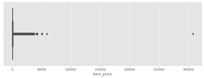
Note: We can count how many items have a price tag above 150000.
train[train['item_price'] > 150000]
| date | date_block_num | shop_id | item_id | item_price | item_cnt_day | item_name | item_category_id | shop_name | item_category_name | |
|---|---|---|---|---|---|---|---|---|---|---|
| 1163158 | 2013-12-13 | 11 | 12 | 6066 | 307980.0 | 1.0 | Radmin 3 - 522 лиц. | 75 | Интернет-магазин ЧС | Программы - Для дома и офиса |
Let’s see if this item has had a difference price previously:
train[train['item_id'] == 6066]
| date | date_block_num | shop_id | item_id | item_price | item_cnt_day | item_name | item_category_id | shop_name | item_category_name | |
|---|---|---|---|---|---|---|---|---|---|---|
| 1163158 | 2013-12-13 | 11 | 12 | 6066 | 307980.0 | 1.0 | Radmin 3 - 522 лиц. | 75 | Интернет-магазин ЧС | Программы - Для дома и офиса |
We can drop this item since this high price appears to be an error.
# remove the single outlier for large price
train = train[train['item_price'] < 150000]
Does the dataset contain negative prices?
train['item_price'].value_counts().sort_index().head()
-1.0000       1
 0.0700       2
 0.0875       1
 0.0900       1
 0.1000    2932
Name: item_price, dtype: int64
Note: One item has a negative price, we remove it from the list.
# remove the single outlier for negative price
train = train[train['item_price'] >= 0]
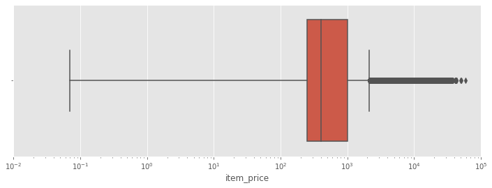
# plot boxplot
f, ax = plt.subplots(figsize=(12, 4))
ax.set_xlim(0.01, 1e5)
ax.set_xscale("log")
sns.boxplot(train['item_price'])
<matplotlib.axes._subplots.AxesSubplot at 0x1a1773acd0>
# plot boxplot
f, ax = plt.subplots(figsize=(12, 4))
sns.boxplot(train['item_cnt_day'])
<matplotlib.axes._subplots.AxesSubplot at 0x1a78fcdfd0>
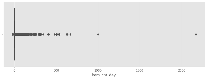
train[train['item_cnt_day'] > 1500]
| date | date_block_num | shop_id | item_id | item_price | item_cnt_day | item_name | item_category_id | shop_name | item_category_name | |
|---|---|---|---|---|---|---|---|---|---|---|
| 2909818 | 2015-10-28 | 33 | 12 | 11373 | 0.908714 | 2169.0 | Доставка до пункта выдачи (Boxberry) | 9 | Интернет-магазин ЧС | Доставка товара |
This day does not correspond to a holiday during which we could expect a large sale. We remove this value.
# remove the outlier for item_cnt_day
train = train[train['item_cnt_day'] < 1500]
fig, ax = plt.subplots(figsize=(12, 12))
sns.scatterplot(x='item_cnt_day', y='item_price', data=train, alpha=0.3)
<matplotlib.axes._subplots.AxesSubplot at 0x1a29353a10>
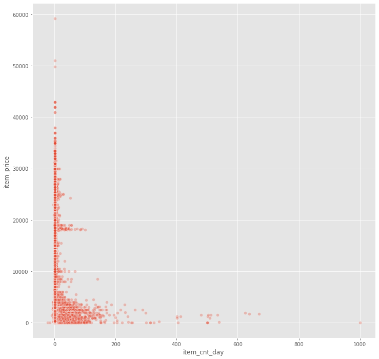
As expected, expensive items are not often purchased. Let’s now inspect trends over time.
EDA Categorical Features
We start by looking for duplicates in the categories. Based on the configuration of the
shops['shop_name'].value_counts().sort_values(ascending=False).head()
Химки ТЦ "Мега"                  1
!Якутск Орджоникидзе, 56 фран    1
Уфа ТЦ "Семья" 2                 1
Калуга ТРЦ "XXI век"             1
Якутск ТЦ "Центральный"          1
Name: shop_name, dtype: int64
There are no obvious duplicates. However, upon detailed inspection of the shop_name feature, we can make the following observations:
- The
shop_namecontains the city of the store. The string is structured as “city, store name” - Several id appears to be duplicates.
The indexes below appear to be duplicates. They are combined under a single index. The same process is applied to the test set.
shops['shop_name'].str.strip('!').sort_values()
2                                    Адыгея ТЦ "Мега"
3                      Балашиха ТРК "Октябрь-Киномир"
4                            Волжский ТЦ "Волга Молл"
5                              Вологда ТРЦ "Мармелад"
6                          Воронеж (Плехановская, 13)
7                              Воронеж ТРЦ "Максимир"
8                        Воронеж ТРЦ Сити-Парк "Град"
9                                   Выездная Торговля
10                         Жуковский ул. Чкалова 39м?
11                         Жуковский ул. Чкалова 39м²
12                                Интернет-магазин ЧС
13                                Казань ТЦ "Бехетле"
14                            Казань ТЦ "ПаркХаус" II
15                               Калуга ТРЦ "XXI век"
16                                   Коломна ТЦ "Рио"
17                      Красноярск ТЦ "Взлетка Плаза"
18                               Красноярск ТЦ "Июнь"
19                              Курск ТЦ "Пушкинский"
20                                Москва "Распродажа"
21                             Москва МТРЦ "Афи Молл"
22                                 Москва Магазин С21
23                   Москва ТК "Буденовский" (пав.А2)
24                   Москва ТК "Буденовский" (пав.К7)
25                                Москва ТРК "Атриум"
26                        Москва ТЦ "Ареал" (Беляево)
27                     Москва ТЦ "МЕГА Белая Дача II"
28                    Москва ТЦ "МЕГА Теплый Стан" II
29                 Москва ТЦ "Новый век" (Новокосино)
30                             Москва ТЦ "Перловский"
31                            Москва ТЦ "Семеновский"
32                         Москва ТЦ "Серебряный Дом"
33                                  Мытищи ТРК "XL-3"
34                               Н.Новгород ТРЦ "РИО"
35                        Н.Новгород ТРЦ "Фантастика"
36              Новосибирск ТРЦ "Галерея Новосибирск"
37                              Новосибирск ТЦ "Мега"
38                                     Омск ТЦ "Мега"
39              РостовНаДону ТРК "Мегацентр Горизонт"
40    РостовНаДону ТРК "Мегацентр Горизонт" Островной
41                             РостовНаДону ТЦ "Мега"
42                             СПб ТК "Невский Центр"
43                                    СПб ТК "Сенная"
44                                Самара ТЦ "Мелодия"
45                               Самара ТЦ "ПаркХаус"
46                              Сергиев Посад ТЦ "7Я"
47                             Сургут ТРЦ "Сити Молл"
48                       Томск ТРЦ "Изумрудный Город"
49                              Тюмень ТРЦ "Кристалл"
50                                 Тюмень ТЦ "Гудвин"
51                          Тюмень ТЦ "Зеленый Берег"
52                               Уфа ТК "Центральный"
53                                   Уфа ТЦ "Семья" 2
54                                    Химки ТЦ "Мега"
55                           Цифровой склад 1С-Онлайн
56                               Чехов ТРЦ "Карнавал"
57                            Якутск Орджоникидзе, 56
0                        Якутск Орджоникидзе, 56 фран
58                            Якутск ТЦ "Центральный"
1                        Якутск ТЦ "Центральный" фран
59                             Ярославль ТЦ "Альтаир"
Name: shop_name, dtype: object
The pairs are defined as (0, 57), (1, 58), (10, 11).
shops['shop_name'].loc[[0, 57, 1, 58, 10, 11]]
0     !Якутск Орджоникидзе, 56 фран
57          Якутск Орджоникидзе, 56
1     !Якутск ТЦ "Центральный" фран
58          Якутск ТЦ "Центральный"
10       Жуковский ул. Чкалова 39м?
11       Жуковский ул. Чкалова 39м²
Name: shop_name, dtype: object
# (0, 57) -> Якутск Орджоникидзе, 56
train.loc[train['shop_id'] == 0, 'shop_id'] = 57
sales_test.loc[sales_test['shop_id'] == 0, 'shop_id'] = 57

# (1, 58) -> Якутск ТЦ "Центральный"
train.loc[train['shop_id'] == 1, 'shop_id'] = 58
sales_test.loc[sales_test['shop_id'] == 1, 'shop_id'] = 58

# (10, 11) -> Жуковский ул. Чкалова 39м²
train.loc[train['shop_id'] == 10, 'shop_id'] = 11
sales_test.loc[sales_test['shop_id'] == 10, 'shop_id'] = 11
# add revenue to train set
train['revenue'] = train['item_price'] * train['item_cnt_day']
train.columns
Index(['date', 'date_block_num', 'shop_id', 'item_id', 'item_price',
       'item_cnt_day', 'item_name', 'item_category_id', 'shop_name',
       'item_category_name', 'revenue'],
      dtype='object')
In addition, we can create a new feature containing the city name associated to the store name.
# replace one faulty city name (Сергиев Посад)
shops.loc[shops['shop_name']=='Сергиев Посад ТЦ "7Я"', 'shop_name'] = 'СергиевПосад ТЦ "7Я"'

# split shop name (and remove the leading !)
shops['city'] = shops['shop_name'].str.strip('!').str.split(' ').map(lambda x: x[0])
shops['city'].value_counts().sort_index()
Адыгея               1
Балашиха             1
Волжский             1
Вологда              1
Воронеж              3
Выездная             1
Жуковский            2
Интернет-магазин     1
Казань               2
Калуга               1
Коломна              1
Красноярск           2
Курск                1
Москва              13
Мытищи               1
Н.Новгород           2
Новосибирск          2
Омск                 1
РостовНаДону         3
СПб                  2
Самара               2
СергиевПосад         1
Сургут               1
Томск                1
Тюмень               3
Уфа                  2
Химки                1
Цифровой             1
Чехов                1
Якутск               4
Ярославль            1
Name: city, dtype: int64
The city name can be encoded to facilitate the use of this feature.
shops['city_id'] = LabelEncoder().fit_transform(shops['city'])
We can now delete the unnecessary columns city and shop_name.
shops = shops[['shop_id', 'city_id']]
The next categorical feature to process is the item category. It is encoded as an id and as a name. The first step consists of looking at the item_category_name to identify potential embedded information.
item_categories.head(10)
| item_category_name | item_category_id | |
|---|---|---|
| 0 | PC - Гарнитуры/Наушники | 0 |
| 1 | Аксессуары - PS2 | 1 |
| 2 | Аксессуары - PS3 | 2 |
| 3 | Аксессуары - PS4 | 3 |
| 4 | Аксессуары - PSP | 4 |
| 5 | Аксессуары - PSVita | 5 |
| 6 | Аксессуары - XBOX 360 | 6 |
| 7 | Аксессуары - XBOX ONE | 7 |
| 8 | Билеты (Цифра) | 8 |
| 9 | Доставка товара | 9 |
It seems that the category contains two components:
- A type
- A subtype
# split `item_category_name`
item_categories['split'] = item_categories['item_category_name'].str.split(' - ')

# isolate `type_name` and 'subtype_name'
item_categories['type_name'] = item_categories['split'].apply(lambda x: x[0].strip())
item_categories['subtype_name'] = item_categories['split'].apply(lambda x: x[1].strip() if len(x)>1 else x[0].strip())

# the type and subtype can be encoded
item_categories['type_id'] = LabelEncoder().fit_transform(item_categories['type_name'])
item_categories['subtype_id'] = LabelEncoder().fit_transform(item_categories['subtype_name'])

# filter out text features
item_categories = item_categories[['item_category_id', 'type_id', 'subtype_id']]
Finally, we apply a similar process to the item names. Since the item names are not consistently defined, we keep only the item_it and the item_category_id.
items = items[['item_id', 'item_category_id']]
Monthly Data
This competition is special because it requires to perform some aggregation on the train set before building the model. In order to make monthly predictions, we aggregate the train set by shop and item. In addition, the train set needs to contain similar shop/item pairs as the test set.
print("=====  ITEMS  =====")
print("There are {} unique items in the train set.".format(len(train['item_id'].unique())))
print("There are {} unique items in the test set.".format(len(sales_test['item_id'].unique())))
print("{} items are in the test but not in the train set.".format(len(set(sales_test['item_id'].unique()) - set(train['item_id'].unique()))))

print("\n===== SHOPS  =====")
print("There are {} unique shops in the train set.".format(len(train['shop_id'].unique())))
print("There are {} unique shops in the test set.".format(len(sales_test['shop_id'].unique())))
print("{} shop are in the test but not in the train set.".format(len(set(sales_test['shop_id'].unique()) - set(train['shop_id'].unique()))))

print("\n===== TEST  =====")
print("The test set contains {} pairs.".format(sales_test.shape[0]))
print("There are {} possible unique pairs using the test data.".format(len(sales_test['item_id'].unique()) * len(sales_test['shop_id'].unique())))
=====  ITEMS  =====
There are 21806 unique items in the train set.
There are 5100 unique items in the test set.
363 items are in the test but not in the train set.

===== SHOPS  =====
There are 57 unique shops in the train set.
There are 42 unique shops in the test set.
0 shop are in the test but not in the train set.

===== TEST  =====
The test set contains 214200 pairs.
There are 214200 possible unique pairs using the test data.
Before we dive into the monthly trends, we need to establish some important rules to help capture the proper sale trends. We need to aggregate the data per month (date_block_num, shop_id, item_id).
from itertools import product
full_data = []
cols = ['date_block_num','shop_id','item_id']

for i in range(34):

    # isolate sales made on ith month
    monthly_sales = train[train['date_block_num']==i]

    # create pairs of id, shops, items
    full_data.append(np.array(list(product([i],
                                        monthly_sales['shop_id'].unique(),
                                        monthly_sales['item_id'].unique())
                               ), dtype='int16'))

# create dataframe
full_data = pd.DataFrame(np.vstack(full_data), columns=cols)

# convert data to optimize memory
full_data['date_block_num'] = full_data['date_block_num'].astype(np.int8)
full_data['shop_id'] = full_data['shop_id'].astype(np.int8)
full_data['item_id'] = full_data['item_id'].astype(np.int16)

# sort values
full_data =  full_data.sort_values(cols)
full_data.shape
(10913804, 3)
The data now needs to be populated. To do so, we compute the aggregates over shop_id, date_block_num, and item_id.
full_data.head()
| date_block_num | shop_id | item_id | |
|---|---|---|---|
| 114910 | 0 | 2 | 19 |
| 117150 | 0 | 2 | 27 |
| 120623 | 0 | 2 | 28 |
| 118316 | 0 | 2 | 29 |
| 114602 | 0 | 2 | 32 |
# aggregate item_cnt_day
monthly_train = train.groupby(['date_block_num','shop_id','item_id']).agg({'item_cnt_day':'sum'})

# reset index and columns
monthly_train = monthly_train.reset_index()

# combine monthly train and pairs
full_data = pd.merge(left=full_data, right=monthly_train, on=cols, how='left')

# clip data, fill nulls with 0, and downsize the datatype
full_data['item_cnt_day'] = full_data['item_cnt_day'].fillna(0).clip(0,20).astype(np.float32)
Include the test set records.
# create month number
sales_test['date_block_num'] = 34

# downsize features
sales_test['shop_id'] = sales_test['shop_id'].astype(np.int16)
sales_test['item_id'] = sales_test['item_id'].astype(np.int16)
sales_test['date_block_num'] = sales_test['date_block_num'].astype(np.int16)

sales_test = sales_test.set_index('ID')
# concat test and full_data
full_data = pd.concat([full_data, sales_test], ignore_index=True, keys=cols, sort=False)

# fill test values to 0
full_data = full_data.fillna(0)
Now that our dataset contains the full sets of month/shop/item, we can add our additional features to complete the set.
# shops
full_data = pd.merge(left=full_data, right=shops, how='left', on='shop_id')

# items
full_data = pd.merge(left=full_data, right=items, how='left', on='item_id')

# item_categories
full_data = pd.merge(left=full_data, right=item_categories, how='left', on='item_category_id')
# downsize the in64
full_data['city_id'] = full_data['city_id'].astype(np.int16)
full_data['item_category_id'] = full_data['item_category_id'].astype(np.int16)
full_data['type_id'] = full_data['type_id'].astype(np.int16)
full_data['subtype_id'] = full_data['subtype_id'].astype(np.int16)
full_data.head()
| date_block_num | shop_id | item_id | item_cnt_day | city_id | item_category_id | type_id | subtype_id | |
|---|---|---|---|---|---|---|---|---|
| 0 | 0 | 2 | 19 | 0.0 | 0 | 40 | 11 | 6 |
| 1 | 0 | 2 | 27 | 1.0 | 0 | 19 | 5 | 12 |
| 2 | 0 | 2 | 28 | 0.0 | 0 | 30 | 8 | 57 |
| 3 | 0 | 2 | 29 | 0.0 | 0 | 23 | 5 | 18 |
| 4 | 0 | 2 | 32 | 0.0 | 0 | 40 | 11 | 6 |
At this point, we have combined our datasets and are ready for more exploration. One of the most common mistake made when performing EDA is to not clearly define what one is trying to archive. In order to avoid this lack of direction, let’s ask ourselves a few questions that we want answer before going further with our dataset.
- What is the monthly total count trend?
- Is there a cycle when averaging the total counts by month?
- What categories are the most sold?
- What shops sell more?
- What categories are generating the most revenue?
- How frequent are returns?
What is the monthly total count trend?
# generate ticks for monthly plots
x_tick_vals = pd.Series(pd.date_range('2013', freq='M', periods=34))
x_tick_vals = [str(x.month) + '/' + str(x.year) for x in x_tick_vals]
groups = full_data.groupby(['date_block_num'])['item_cnt_day'].sum()
fig, ax = plt.subplots(figsize=(14,6))
ax.set_title('Total item sold')
ax.set_ylim(0,groups.max())
ax.set_xlabel('Date')
ax.set_xticks(range(34))
ax.set_xticklabels(x_tick_vals, rotation=60)
ax.plot(groups[:-1]);
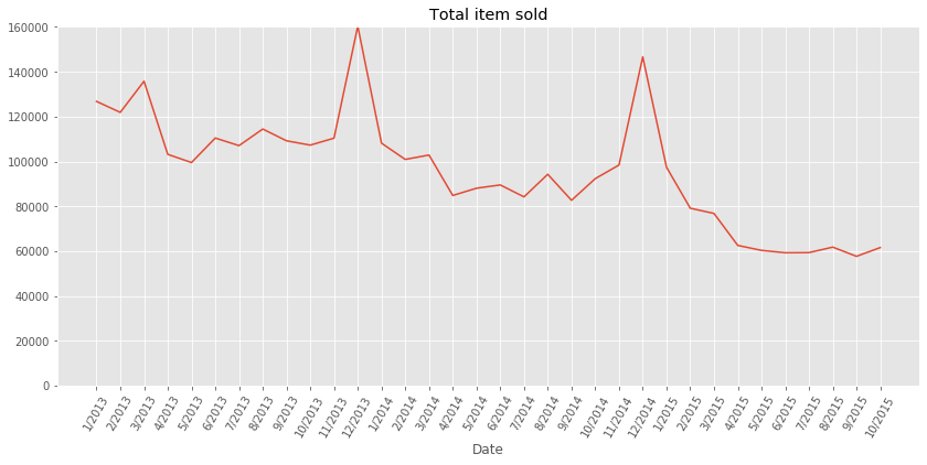
Note: From the above plot, we can make two observations:
- There seems to be a overall decrease of sales year after year
- The plot present some seasonality, the sales during the month of December are much higher that the sales during the preceding and following months. This can be explained as the Holiday season is typically prone to more spendings.
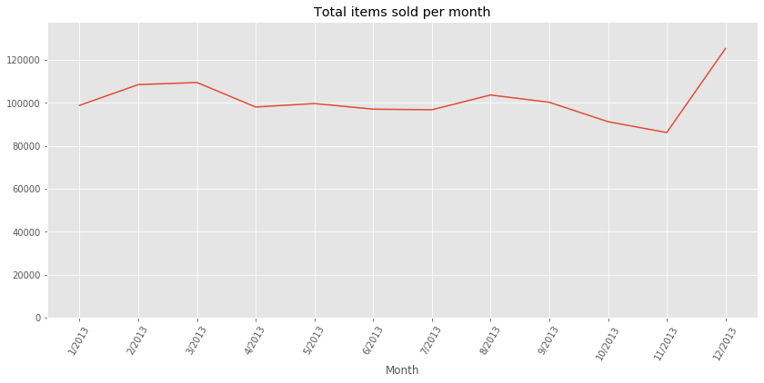
Is there a cycle when averaging the total counts by month?
train['month'] = train['date'].dt.month
train['year'] = train['date'].dt.year
groups = train.groupby(['year','month'])['item_cnt_day'].sum()
groups = groups.reset_index()
groups = groups.groupby('month')['item_cnt_day'].mean()
fig, ax = plt.subplots(figsize=(14,6))
ax.set_title('Total items sold per month')
ax.set_ylim(0,1.1*groups.max())
ax.set_xlabel('Month')
ax.set_xticks(range(1,13))
ax.set_xticklabels(x_tick_vals, rotation=60)
ax.plot(groups);
What categories are the most sold?
gp_category_mean = full_data.groupby(['item_category_id'], as_index=False)['item_cnt_day'].mean()
gp_category_sum = full_data.groupby(['item_category_id'], as_index=False)['item_cnt_day'].sum()
f, axes = plt.subplots(2, 1, figsize=(16, 10), sharex=True)
sns.barplot(x="item_category_id", y="item_cnt_day", data=gp_category_mean, ax=axes[0], palette="deep").set_title("Average number of item sold daily per category")
sns.barplot(x="item_category_id", y="item_cnt_day", data=gp_category_sum, ax=axes[1], palette="deep").set_title("Average number of item sold per category")
axes[0].set_xlabel('')
axes[1].set_xticklabels(axes[1].get_xticklabels(), rotation=60)
axes[1].tick_params(labelsize=8)
plt.show()
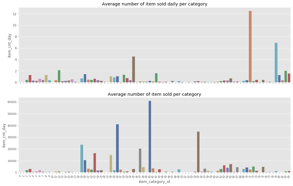
Note: From the above two plots, we can observer two interesting facts:
- The sales are clearly unbalances amongst item categories. Several categories (71 and 79) account for a very large portion of the average daily item category count sold daily.
a. “Подарки - Сумки, Альбомы, Коврики д/мыши”,71 (Gifts - Bags, Albums, Mousepads)
b. Служебные,79 (Office furnitures) - When looking at the average number of item sold per categories, new categories appear to dominate the sales.
a. Игры PC - Стандартные издания,30 (PC Games - Standard Editions)
b. Кино - DVD,40 (Cinema - DVD)
c. Музыка - CD локального производства,55 (Music - Local Production CD)
The discrepancy between the two plots can be explained because not all the items and all the categories were sold during the entire timeframe of the study.
What shops sell more?
gp_shops_sum = full_data.groupby(['shop_id'], as_index=False)['item_cnt_day'].sum()
f, ax = plt.subplots(figsize=(16, 8))
sns.barplot(x="shop_id", y="item_cnt_day", data=gp_shops_sum, ax=ax, palette="deep").set_title("Total number of item sold per store")
ax.set_xlabel('')
ax.set_xticklabels(axes[1].get_xticklabels(), rotation=60)
ax.tick_params(labelsize=8)
plt.show()
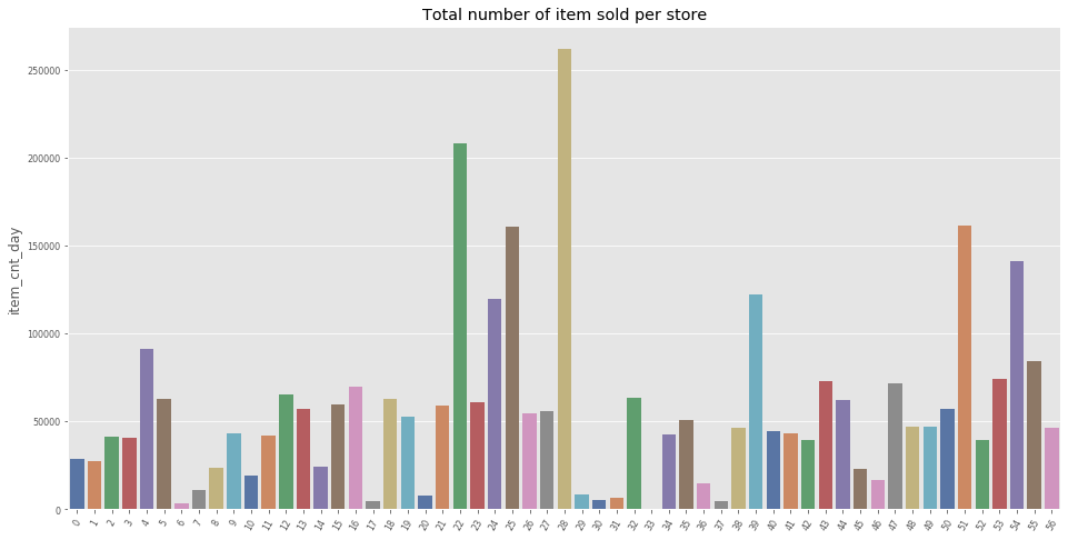
Note: From the above plots, we can see a wide distribution of item sold per store. This can be a helpful feature as the size of the store is certainly correlated to the monthly sales of each items.
What categories are generating the most revenue?
gp_cat_rev = train.groupby(['year', 'item_category_id'], as_index=False)['revenue'].sum()
sns.catplot(x="item_category_id", y="revenue",
            data=gp_cat_rev, row="year",
            palette="deep", kind="bar",
            height=4, aspect=3.5)
plt.show()
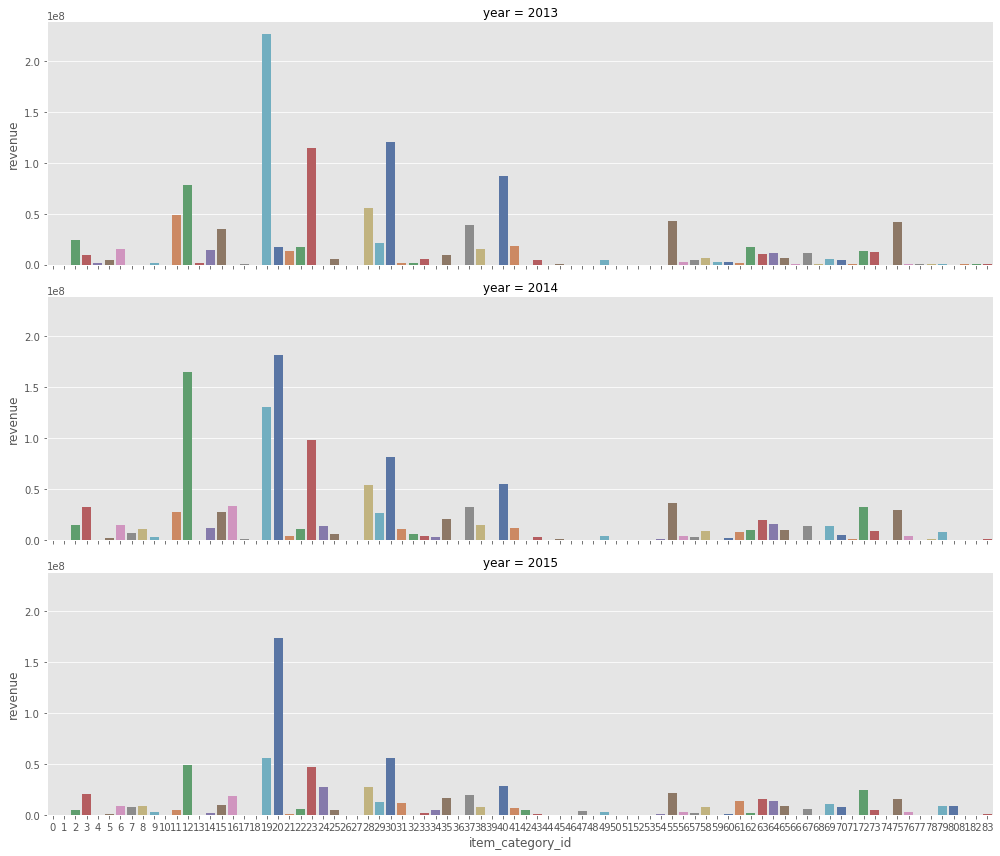
Note: The above plots help understand two important aspects of the sale trends:
- There is a time effect related to what item categories are popular. For instance, in 2013, the category19 was very popular and its associated revenue has been decreasing since.
- As expected, the category feature is directly related to quantities sold.
How frequent are returns?
return_df = train.copy()
return_df['return'] = return_df['item_cnt_day'].apply(lambda x: -min(x, 0))
return_df['sales'] = return_df['item_cnt_day'].apply(lambda x: max(x, 0))
Return per category
return_cats = return_df.groupby(['item_category_id'], as_index=False)['return', 'sales'].sum()
return_cats['percent_return'] = return_cats['return'] / return_cats['sales'] * 100.
f, ax = plt.subplots(figsize=(16, 8))
sns.barplot(x="item_category_id", y="percent_return", data=return_cats, ax=ax, palette="deep").set_title("Percentage of return per category")
ax.set_xlabel('')
ax.set_xticklabels(axes[1].get_xticklabels(), rotation=60)
ax.tick_params(labelsize=8)
plt.show()
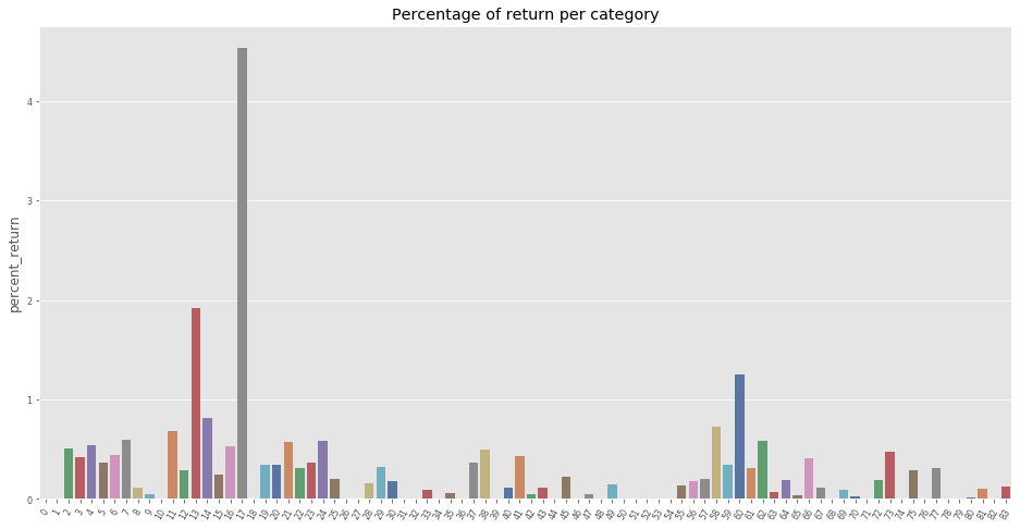
Note: From the above, we can see that the item category 17 (Игровые консоли - Прочие, Game consoles - Other) experiences the highest rate of return (4.5%). This is helpful because this feature can be use to better predict the quantity returned every month.
Return per store
return_stores = return_df.groupby(['shop_id'], as_index=False)['return', 'sales'].sum()
return_stores['percent_return'] = return_stores['return'] / return_stores['sales'] * 100.
f, ax = plt.subplots(figsize=(16, 8))
sns.barplot(x="shop_id", y="percent_return", data=return_stores, ax=ax, palette="deep").set_title("Return rate per store")
ax.set_xlabel('')
ax.set_xticklabels(axes[1].get_xticklabels(), rotation=60)
ax.tick_params(labelsize=8)
plt.show()
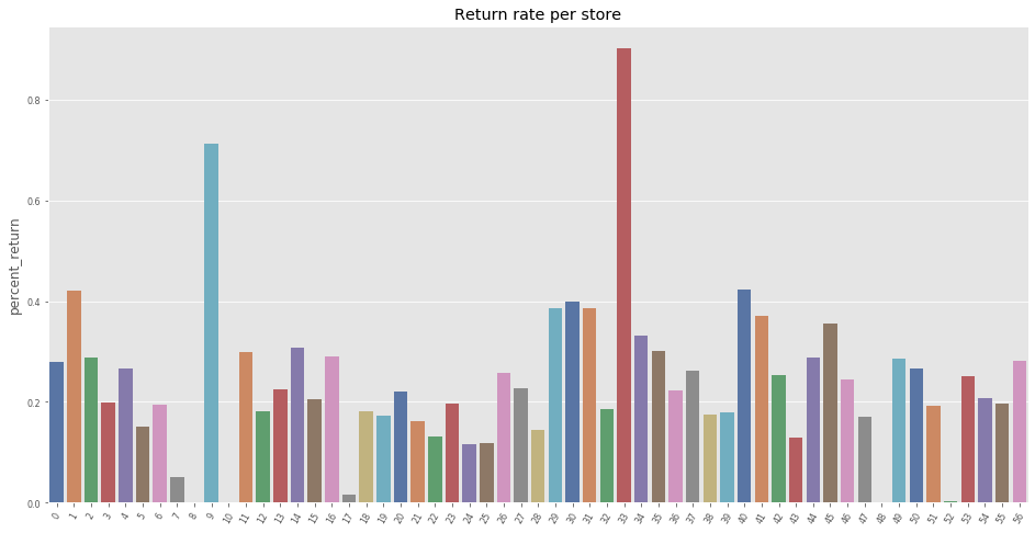
Note: The above plot shows that overall, the shops experience a similar rate of return (~0.4%). However, two stores (9 and 33) experience a higher rate of return with 0.7% and 0.85% respectively.
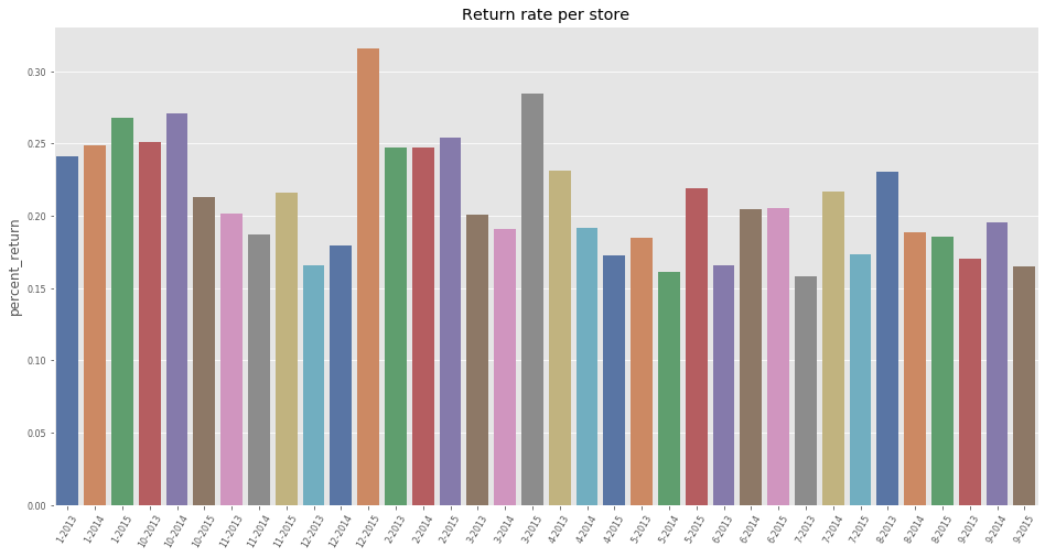
Return per month
return_df['date'] = return_df['month'].astype('str').str.cat(return_df['year'].astype('str'),sep="-")
return_month = return_df.groupby(['date'], as_index=False)['return', 'sales'].sum()
return_month['percent_return'] = return_month['return'] / return_month['sales'] * 100.
f, ax = plt.subplots(figsize=(16, 8))
sns.barplot(x="date", y="percent_return", data=return_month, ax=ax, palette="deep").set_title("Return rate per store")
ax.set_xlabel('')
ax.set_xticklabels(ax.get_xticklabels(), rotation=60)
ax.tick_params(labelsize=8)
plt.show()
Before performing some feature engineering, we clean up the memory of unused variables.
del ax, axes
del bench_oct2015, test_oct2015, test_submission
del f, fig, x_tick_vals
del i
del gp_cat_rev, gp_category_mean, gp_category_sum, gp_shops_sum, groups
del return_cats, return_stores, monthly_train, monthly_sales
Feature Engineering
In this section, we leverage the valuable insights we obtained from the EDA by creating new features. The first step consists of creating a function to help generate lag features. For instance, we want each monthly record to contain information about the sales from the n-th previous month.
Downcast
In order to save some memory, we downcast the floats and integers stored in the dataset.
print('Datasize before downcast:')
print(full_data.info())
Datasize before downcast:
<class 'pandas.core.frame.DataFrame'>
Int64Index: 11128004 entries, 0 to 11128003
Data columns (total 8 columns):
date_block_num      int16
shop_id             int16
item_id             int16
item_cnt_day        float32
city_id             int16
item_category_id    int16
type_id             int16
subtype_id          int16
dtypes: float32(1), int16(7)
memory usage: 275.9 MB
None
def downcast_dtypes(df):
    '''
        Changes column types in the dataframe:

                `float64` type to `float16`
                `int64`   type to `int16`http://localhost:8888/notebooks/Google%20Drive/2-Coding/1-Coursera/Advanced%20ML/2-Kaggle/Final%20Project/Final%20Project.ipynb#
    '''

    # Select columns to downcast
    float_cols = [c for c in df if df[c].dtype == "float64" or df[c].dtype == 'float32']
    int_cols =   [c for c in df if (df[c].dtype == "int64" or df[c].dtype == 'int32'  or df[c].dtype == 'int16') and (c!='item_id')]

    # Downcast
    df[float_cols] = df[float_cols].astype(np.float16)
    df[int_cols]   = df[int_cols].astype(np.int8)

    return df
full_data = downcast_dtypes(full_data)
print('Datasize after downcast:')
print(full_data.info())
Datasize after downcast:
<class 'pandas.core.frame.DataFrame'>
Int64Index: 11128004 entries, 0 to 11128003
Data columns (total 8 columns):
date_block_num      int8
shop_id             int8
item_id             int16
item_cnt_day        float16
city_id             int8
item_category_id    int8
type_id             int8
subtype_id          int8
dtypes: float16(1), int16(1), int8(6)
memory usage: 191.0 MB
None
New Features and Encoding
Before we implement the lags, we need to define what features we want to lag. Based on the EDA, the following features will be used:
- Per shop_id and item_id, we want to propagate the min, average, and max price
- Per shop_id and item id, we want to propagate the current streak of sales (in month)
- Per store_id, item_id, we want the number of returns
- Per item_id, we want to propagate the min, average, and max price
- Per item_id, we want the number of store selling the item
- Per shop_id, we want the number of item sold
- Per shop_id, we want the most famous category
# create return features
return_df = return_df[['date_block_num', 'shop_id', 'item_id', 'item_category_id', 'return']]
# ===========================
# create groups
# ===========================

# items
group_item = full_data.groupby(['date_block_num','item_id'], as_index=False)

# store + item
group_store_item = full_data.groupby(['date_block_num','item_id', 'shop_id'], as_index=False)

# store
group_store = full_data.groupby(['date_block_num', 'shop_id'])

# category
group_cat = full_data.groupby(['date_block_num', 'item_category_id'])

# category + store
group_cat_store = full_data.groupby(['date_block_num', 'shop_id', 'item_category_id'])

# type code
group_type = full_data.groupby(['date_block_num', 'type_id'])

# type + store
group_type_shop = full_data.groupby(['date_block_num', 'shop_id', 'type_id'])

# subtype
group_subtype = full_data.groupby(['date_block_num', 'subtype_id'])

# subtype + store
group_subtype_shop = full_data.groupby(['date_block_num', 'shop_id', 'subtype_id'])

# city
group_city = full_data.groupby(['date_block_num', 'city_id'])

# city + item
group_city_item = full_data.groupby(['date_block_num', 'item_id', 'city_id'])

# return per shop + item
return_shop_item = return_df.groupby(['date_block_num', 'shop_id', 'item_id'], as_index=False).agg(np.sum)

# return per shop
return_shop = return_df.groupby(['date_block_num', 'shop_id'], as_index=False)['return'].agg(np.sum)

# return per item
retun_item = return_df.groupby(['date_block_num', 'item_id'], as_index=False)['return'].agg(np.sum)

# ===========================
# create encodings
# ===========================

# PRICE
# min, max, average of price per items per month
monthly_sales_group = train.groupby(['date_block_num','item_id'])
min_max_avg_prices = monthly_sales_group['item_price'].agg(['min', 'max', np.mean]).reset_index()
min_max_avg_prices = min_max_avg_prices.rename(columns={"min": "min_item_price",
                                                        "max": "max_item_price",
                                                        "mean": "avg_item_price"})

# min, max, average of price per item per item per store per month
monthly_sales_item_store_group = train.groupby(['date_block_num','item_id', 'shop_id'])
min_max_avg_item_store = monthly_sales_item_store_group['item_price'].agg(['min', 'max', np.mean]).reset_index()
min_max_avg_item_store = min_max_avg_item_store.rename(columns={"min": "min_item_shop_price",
                                                                "max": "max_item_shop_price",
                                                                "mean": "avg_item_shop_price"})

# RETURNS
# sum returns per store
return_shop = return_df.groupby(['date_block_num', 'shop_id'], as_index=False)['return'].agg(np.sum).rename(columns={'return': "shop_return"})

# sum returns per item
return_item = return_df.groupby(['date_block_num', 'item_id'], as_index=False)['return'].agg(np.sum).rename(columns={'return': "item_return"})

# sum returns per category
return_cat = return_df.groupby(['date_block_num', 'item_category_id'], as_index=False)['return'].agg(np.sum).rename(columns={'return': "cat_return"})

# sum returns per store + item
return_item_store = return_df.groupby(['date_block_num', 'item_id', 'shop_id'], as_index=False)['return'].agg(np.sum).rename(columns={'return': "item_shop_return"})

# sum returns per store per category
return_store_cat = return_df.groupby(['date_block_num', 'shop_id', 'item_category_id'], as_index=False)['return'].agg(np.sum).rename(columns={'return': "cat_shop_return"})

# SALES
# number of stores selling the item per month
store_count = full_data.groupby(['date_block_num','item_id'])['shop_id'].count().reset_index()
store_count = store_count.rename(columns={'shop_id': "shop_count"})

# target item count
target_item = full_data.groupby(['date_block_num', 'item_id'], as_index=False)['item_cnt_day'].sum()
target_item = target_item.rename(columns={"item_cnt_day": "item_sold"})

# number of unique items sold in store per month
unique_items = group_store['item_id'].nunique().reset_index()
unique_items = unique_items.rename(columns={'item_id': "item_avail"})

# number of item sold per category
cat_count = group_cat['item_cnt_day'].agg(np.mean).reset_index()
cat_count = cat_count.rename(columns={'item_cnt_day': 'avg_cat_count'})

# nunber of item sold per category per store
cat_store_count = group_cat_store['item_cnt_day'].agg(np.mean).reset_index()
cat_store_count = cat_store_count.rename(columns={'item_cnt_day': 'avg_cat_store_count'})

# TYPES AND SUBTYPES
# types
type_count = group_type['item_cnt_day'].agg(np.mean).reset_index()
type_count = type_count.rename(columns={'item_cnt_day':'avg_type'})

type_store_count = group_type_shop['item_cnt_day'].agg(np.mean).reset_index()
type_store_count = type_store_count.rename(columns={'item_cnt_day':'avg_type_store'})

# subtype
subtype_count = group_subtype['item_cnt_day'].agg(np.mean).reset_index()
subtype_count = subtype_count.rename(columns={'item_cnt_day':'avg_subtype'})

subtype_store_count = group_subtype_shop['item_cnt_day'].agg(np.mean).reset_index()
subtype_store_count = subtype_store_count.rename(columns={'item_cnt_day':'avg_subtype_store'})

# CITY
city_count = group_city['item_cnt_day'].agg(np.mean).reset_index().rename(columns={'item_cnt_day':'avg_city'})
city_count_item = group_city_item['item_cnt_day'].agg(np.mean).reset_index().rename(columns={'item_cnt_day':'avg_city_item'})
In addition to the encoded features, we need a function to compute streaks. Three streaks are considered:
- Number of successive month the item has been sold (looking only at the previous months).
- Number of total sales for the item.
- Number of total sales for the item with a 0 for month during which sales=0.
def streak(df, col):
    """
    Return a new feature corresponding to the streak of the sales for an item.
    """

    clone = df[['item_id', 'shop_id', 'date_block_num', col]].copy()

    # sort clone (item_id, shop_id, data_block_num)
    clone = clone.sort_values(['item_id', 'shop_id', 'date_block_num'])

    # create new sold feature
    clone['sold'] = (clone[col] > 0).astype(int)

    # create streak reset condition
    reset = (clone['sold']!=clone['sold'].shift()) | \
            (clone['item_id']!=clone['item_id'].shift()) | \
            (clone['shop_id']!=clone['shop_id'].shift())

    # create streak
    clone['streak'] = clone['sold'].groupby((reset).cumsum()).cumsum()

    # add total sales (10, 11, 0, 0, 5, 1, 0) => (10, 21, 21, 21, 26, 27, 27)
    cum_sales_df = clone.groupby(
        by=['item_id', 'shop_id', 'date_block_num'])[col].sum().groupby(
            level=[0, 1]).cumsum().reset_index().rename(
                columns={col: 'cum_sales'})
    clone = pd.merge(left=clone,
                     right=cum_sales_df,
                     on=['item_id', 'shop_id', 'date_block_num'],
                     how='left')

    # delete column
    del clone[col]

    # merge streak with original df
    return_df = pd.merge(left=df,
                         right=clone,
                         on=['item_id', 'shop_id', 'date_block_num'],
                         how='left')

    # add sale streak in term of number (10, 11, 0, 0, 5, 1, 0) => (10, 21, 0, 0, 5, 6, 0)
    return_df['cum_if_sales'] = return_df['cum_sales']

    # remove values of cum_if_sales for months without sales
    return_df['cum_if_sales'] = return_df['cum_if_sales'] * return_df['sold']

    # delete column
    del return_df['sold']

    return return_df
# combine all new features with original dataframe and create sale streaks
key_item_store = ['item_id', 'shop_id', 'date_block_num']
key_item = ['item_id', 'date_block_num']
key_store = ['shop_id', 'date_block_num']
key_store_cat = ['shop_id', 'shop_id', 'item_category_id', 'date_block_num']
key_cat = ['item_category_id', 'date_block_num']
key_type = ['type_id', 'date_block_num']
key_type_shop = ['type_id', 'shop_id', 'date_block_num']
key_subype = ['subtype_id', 'date_block_num']
key_subtype_shop = ['subtype_id', 'shop_id', 'date_block_num']
key_city = ['city_id', 'date_block_num']
key_city_item = ['city_id', 'item_id', 'date_block_num']
filename = 'data'
with open(filename, 'wb') as outfile:
    pickle.dump(full_data, outfile)
# PRICE
full_data = pd.merge(left=full_data, right=min_max_avg_prices, on=key_item, how='left')
full_data = pd.merge(left=full_data, right=min_max_avg_item_store, on=key_item_store, how='left')

# RETURNS
full_data = pd.merge(left=full_data, right=return_shop, on=key_store, how='left')
full_data = pd.merge(left=full_data, right=return_item, on=key_item, how='left')
#full_data = pd.merge(left=full_data, right=return_cat, on=key_cat, how='left')
full_data = pd.merge(left=full_data, right=return_item_store, on=key_item_store, how='left')
#full_data = pd.merge(left=full_data, right=return_store_cat, on=key_store_cat, how='left')

# SALES
full_data = pd.merge(left=full_data, right=store_count, on=key_item, how='left')
full_data = pd.merge(left=full_data, right=target_item, on=key_item, how='left')
#full_data = pd.merge(left=full_data, right=unique_items, on=key_store, how='left')
full_data = pd.merge(left=full_data, right=cat_count, on=key_cat, how='left')
full_data = pd.merge(left=full_data, right=cat_store_count, on=key_store_cat, how='left')

# TYPES AND SUBTYPES
full_data = pd.merge(left=full_data, right=type_count, on=key_type, how='left')
full_data = pd.merge(left=full_data, right=type_store_count, on=key_type_shop, how='left')
full_data = pd.merge(left=full_data, right=subtype_count, on=key_subype, how='left')
full_data = pd.merge(left=full_data, right=subtype_store_count, on=key_subtype_shop, how='left')

# CITY
#full_data = pd.merge(left=full_data, right=city_count, on=key_city, how='left')
#full_data = pd.merge(left=full_data, right=city_count_item, on=key_city_item, how='left')
# fill_na
columns = ['min_item_price', 'max_item_price', 'avg_item_price',
           'min_item_shop_price', 'max_item_shop_price', 'avg_item_shop_price',
           'shop_return', 'item_return', 'item_shop_return']

full_data.loc[:, columns] = full_data[columns].fillna(0)

# create data skreak
full_data = streak(full_data, 'item_cnt_day')
del min_max_avg_prices, min_max_avg_item_store, return_shop, return_item, return_cat, return_item_store
del return_store_cat, store_count, target_item, unique_items, cat_count, cat_store_count
del type_count, type_store_count, subtype_count, subtype_store_count
del city_count, city_count_item
del return_df, return_shop_item, return_month
filename = 'data'
with open(filename, 'wb') as outfile:
    pickle.dump(full_data, outfile)
#with open(filename, 'rb') as infile:
#    full_data = pickle.load(infile)
Lags
In order for the past information to be available when making predictions for the current month, lagged features need to be created. They consists of conveying the information from the past to the current records. For instance, what was the number of sales for a specific pair of item and shop during the previous month.
# List of columns that we will use to create lags
index_cols = ['shop_id', 'item_id', 'date_block_num']
no_shift = ['city_id', 'item_category_id', 'subtype_id', 'type_id']
cols_to_rename = list(full_data.columns.difference(index_cols).difference(no_shift))
We can now create a set of lagged features using lags ranging from 1 to 12 months.
def lag_feature(df,lags, cols):
    '''
    Add new lag columns to the dataframe (df).
    Inputs:
        df: input dataframe containing time-series data.
        lags: list of integer corresponding to the desired lags.
    '''
    for month_shift in tqdm_notebook(lags):

        # clone df
        df_shift = df[index_cols + cols].copy()

        # shift date_block_num
        df_shift['date_block_num'] = df_shift['date_block_num'] + month_shift

        # dummy rename function
        foo = lambda x: '{}_lag_{}'.format(x, month_shift) if x in cols else x

        # rename columns
        df_shift = df_shift.rename(columns=foo)

        # downcast
        df_shift = downcast_dtypes(df_shift)

        # merge original data with shift
        df = pd.merge(df, df_shift, on=index_cols, how='left').fillna(0)

    return df
# create lags
full_data = lag_feature(full_data, [1], ['avg_cat_count', 'avg_cat_store_count',
                                         'avg_subtype', 'avg_subtype_store',
                                         'avg_type', 'avg_type_store',
                                         'item_return', 'item_shop_return',
                                         'item_sold', 'shop_count', 'shop_return'])

full_data = lag_feature(full_data, [1,2,3,4], ['min_item_price', 'avg_item_price',
                                               'cum_if_sales', 'cum_sales',
                                               'max_item_price'])

full_data = lag_feature(full_data, [1,2,3,4,5,6], ['max_item_shop_price', 'min_item_shop_price',
                                                   'avg_item_shop_price'])

full_data = lag_feature(full_data, [1,2,3,4,5,6,12], ['item_cnt_day', 'streak'])
HBox(children=(IntProgress(value=0, max=1), HTML(value='')))


HBox(children=(IntProgress(value=0, max=4), HTML(value='')))


HBox(children=(IntProgress(value=0, max=6), HTML(value='')))


HBox(children=(IntProgress(value=0, max=7), HTML(value='')))
# Extract time based features.
full_data['year'] = full_data['date_block_num'].apply(lambda x: ((x//12) + 2013))
full_data['month'] = full_data['date_block_num'].apply(lambda x: (x % 12))
Train / Test Split
The objective of the model is to accurately predict sales of the 34th month. Since the test set is defined in the future of our available dataset, we need to respect the same conditions when defining our train/validation split. That is, the months included in the validation split should be posterior to the train period.
- The training set is defined using months 12 to 28 (we remove the first 12 months as the data may be too old to accurately represent current trends in the sales).
- The validation set is defined using months 29 to 33 and the test set will use block 34.
In addition, the goal of this competition is to predict the sales of month N without any information related to month N. Therefore, we delete from our dataset the features that are related to the sales of the current month.
Purge Features
# metrics related to the sales of current month (to be deleted)
to_delete = [
    "min_item_price", "max_item_price", "avg_item_price",
    "min_item_shop_price", "max_item_shop_price", "avg_item_shop_price",
    "shop_return", "item_return", "item_shop_return", "shop_count",
    "item_sold", "item_avail", "avg_cat_count", "avg_cat_store_count",
    "avg_type", "avg_type_store", "avg_subtype", "avg_subtype_store", "streak",
    "cum_sales", "cum_if_sales"
]
# purge full set of columns to be deleted
full_data = full_data[full_data.columns.difference(to_delete)]
Now we delete the first 12 months worth of data.
# remove first 12 months (null lag and old data)
full_data = full_data[(full_data['date_block_num']>=12)]
filename = 'data_before_split'
with open(filename, 'wb') as outfile:
    pickle.dump(full_data, outfile)
#with open(filename, 'rb') as infile:
#    full_data = pickle.load(infile)
Make Splits
Finally, we split the dataset into a training, a validation, and a test set according to the rules defined above.
# train set
X_train = full_data[full_data['date_block_num'] < 28].drop(['item_cnt_day'],
                                                           axis=1)
X_train_dates = full_data[full_data['date_block_num'] < 28]['date_block_num']
Y_train = full_data[full_data['date_block_num'] < 28]['item_cnt_day']

# validation set for first-layer model
X_valid = full_data[(full_data['date_block_num'] >= 28)
                    & (full_data['date_block_num'] < 33)].drop(
                        ['item_cnt_day'], axis=1)
X_valid_dates = full_data[(full_data['date_block_num'] >= 28)
                    & (full_data['date_block_num'] < 33)]['date_block_num']
Y_valid = full_data[(full_data['date_block_num'] >= 28)
                    & (full_data['date_block_num'] < 33)]['item_cnt_day']

# validation set for meta-model
X_valid_meta = full_data[full_data['date_block_num'] == 33].drop(['item_cnt_day'],axis=1)
X_valid_meta_dates = full_data[full_data['date_block_num'] == 33]['date_block_num']
Y_valid_meta = full_data[full_data['date_block_num'] == 33]['item_cnt_day']

# test set (predictions)
X_test = full_data[full_data['date_block_num'] == 34].drop(['item_cnt_day'],
                                                           axis=1)
We create a checkpoint by pickling our train, validation, and test sets.
# train
pickle.dump(X_train, open('X_train.pickle', 'wb'))
pickle.dump(Y_train, open('Y_train.pickle', 'wb'))
pickle.dump(X_train_dates, open('X_train_dates.pickle', 'wb'))

# validation
pickle.dump(X_valid, open('X_valid.pickle', 'wb'))
pickle.dump(Y_valid, open('Y_valid.pickle', 'wb'))
pickle.dump(X_valid_dates, open('X_valid_dates.pickle', 'wb'))

# validation meta
pickle.dump(X_valid_meta, open('X_valid_meta.pickle', 'wb'))
pickle.dump(Y_valid_meta, open('Y_valid_meta.pickle', 'wb'))
pickle.dump(X_valid_meta_dates, open('X_valid_meta_dates.pickle', 'wb'))

# test
pickle.dump(X_test, open('X_test.pickle', 'wb'))
Validate Split Strategy
# define number of total records
n_rows = X_train.shape[0] + X_valid.shape[0] + X_test.shape[0] + X_valid_meta.shape[0]

# print fractions
print('Train set records:', X_train.shape[0])
print('Validation set records:', X_valid.shape[0])
print('Meta validation set records:', X_valid_meta.shape[0])
print('Test set records:', X_test.shape[0])

print('Train set records: %s (%.f%% of complete data)' % (X_train.shape[0], ((X_train.shape[0]/n_rows)*100)))
print('Validation set records: %s (%.f%% of complete data)' % (X_valid.shape[0], ((X_valid.shape[0]/n_rows)*100)))
print('Meta validation set records: %s (%.f%% of complete data)' % (X_valid_meta.shape[0], ((X_valid_meta.shape[0]/n_rows)*100)))
Train set records: 5068102
Validation set records: 1118820
Meta validation set records: 238172
Test set records: 214200
Train set records: 5068102 (76% of complete data)
Validation set records: 1118820 (17% of complete data)
Meta validation set records: 238172 (4% of complete data)
print('mean for whole train set: {0}'.format(
    np.mean(full_data.loc[full_data['date_block_num'] < 28, 'item_cnt_day'].astype(
        np.float32))))
print('mean for validation train set: {0}'.format(
    np.mean(full_data.loc[(full_data['date_block_num'] < 33) & (full_data['date_block_num'] >= 28), 'item_cnt_day'].astype(
        np.float32))))
mean for whole train set: 0.29374054074287415
mean for validation train set: 0.2667059898376465
Note: the above means are very close to the value obtained by probing the leaderboard.
Since we have been generating a lot of data, it is important to clear unnecessary variable. We have created our train, validation, and test set so the full dataset can be deleted.
Finally, we can look at new records in the test set, that is pairs the set of item_id from the test set not included in the train set.
item_in_test_only = set(X_test['item_id'].unique()).difference(set(X_train['item_id']))
print('Items in test and not in train: {0}'.format(len(item_in_test_only)))
item_in_train_only = set(X_train['item_id'].unique()).difference(set(X_test['item_id']))
print('Items in train and not in test: {0}'.format(len(item_in_train_only)))
Items in test and not in train: 1499
Items in train and not in test: 11626
del full_data
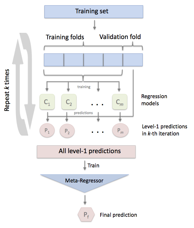
Models
We are now ready to train our models. We are going to follow a typical ensembling process:
- Examine feature importance to see if PCA is needed.
- Create first layer models.
- For the promising base-layer models, fine-tune the hyperparameters.
- Stack model using a meta-model.
Feature Importance
import pickle
import pandas as pd
import numpy as np
import matplotlib.pyplot as plt
import time
import xgboost
from xgboost import XGBRegressor
import gc

gc.collect()
# reload
X_train = pd.read_pickle('X_train.pickle')
X_train_dates = pd.read_pickle('X_train_dates.pickle')
Y_train = pd.read_pickle('Y_train.pickle')

X_valid = pd.read_pickle('X_valid.pickle')
X_valid_dates = pd.read_pickle('X_valid_dates.pickle')
Y_valid = pd.read_pickle('Y_valid.pickle')

X_valid_meta = pd.read_pickle('X_valid_meta.pickle')
X_valid_meta_dates = pd.read_pickle('X_valid_meta_dates.pickle')
Y_valid_meta = pd.read_pickle('Y_valid_meta.pickle')

X_test = pd.read_pickle('X_test.pickle')
In order to obtain the feature importances, we create a simple tree-based model (Random-Forest) and extract the feature importances.
# create simple random forest
forest = ExtraTreesRegressor(n_estimators=50,
                              random_state=0,
                              verbose=1,
                              n_jobs=-1)

# train model on training set
forest.fit(X_train, Y_train)

# extract feature importances
importances = forest.feature_importances_
std = np.std([tree.feature_importances_ for tree in forest.estimators_],
             axis=0)
indices = np.argsort(importances)[::-1]
[Parallel(n_jobs=-1)]: Using backend ThreadingBackend with 4 concurrent workers.
[Parallel(n_jobs=-1)]: Done  42 tasks      | elapsed: 51.8min
[Parallel(n_jobs=-1)]: Done  50 out of  50 | elapsed: 58.1min finished
pd.options.display.max_rows = 999
feature_importance = pd.DataFrame(data = {'feature':X_train.columns,'score_mean':importances,'score_std':std})
feature_importance.sort_values('score_mean', ascending=False)
| feature | score_mean | score_std | |
|---|---|---|---|
| 27 | item_cnt_day_lag_1 | 0.305195 | 0.042668 |
| 34 | item_id | 0.125091 | 0.003394 |
| 60 | shop_id | 0.039580 | 0.002824 |
| 37 | item_sold_lag_1 | 0.038010 | 0.021622 |
| 16 | city_id | 0.027129 | 0.001806 |
| 58 | month | 0.025071 | 0.002134 |
| 29 | item_cnt_day_lag_2 | 0.024382 | 0.027393 |
| 13 | avg_subtype_store_lag_1 | 0.021515 | 0.006218 |
| 69 | subtype_id | 0.021043 | 0.004745 |
| 26 | item_category_id | 0.018220 | 0.004668 |
| 25 | date_block_num | 0.017076 | 0.001475 |
| 15 | avg_type_store_lag_1 | 0.016783 | 0.000826 |
| 1 | avg_cat_store_count_lag_1 | 0.016078 | 0.001597 |
| 30 | item_cnt_day_lag_3 | 0.015121 | 0.008848 |
| 61 | shop_return_lag_1 | 0.013561 | 0.000370 |
| 18 | cum_if_sales_lag_2 | 0.012104 | 0.014885 |
| 17 | cum_if_sales_lag_1 | 0.011855 | 0.017054 |
| 62 | streak_lag_1 | 0.009901 | 0.017725 |
| 31 | item_cnt_day_lag_4 | 0.009412 | 0.008743 |
| 48 | min_item_price_lag_1 | 0.008958 | 0.000425 |
| 59 | shop_count_lag_1 | 0.008888 | 0.000927 |
| 21 | cum_sales_lag_1 | 0.008629 | 0.004356 |
| 14 | avg_type_lag_1 | 0.008317 | 0.000455 |
| 0 | avg_cat_count_lag_1 | 0.008092 | 0.000505 |
| 12 | avg_subtype_lag_1 | 0.008021 | 0.000505 |
| 22 | cum_sales_lag_2 | 0.007750 | 0.006408 |
| 70 | type_id | 0.007607 | 0.001340 |
| 49 | min_item_price_lag_2 | 0.006894 | 0.000784 |
| 2 | avg_item_price_lag_1 | 0.006879 | 0.000407 |
| 32 | item_cnt_day_lag_5 | 0.006349 | 0.001230 |
| 3 | avg_item_price_lag_2 | 0.006176 | 0.000789 |
| 38 | max_item_price_lag_1 | 0.005687 | 0.000350 |
| 52 | min_item_shop_price_lag_1 | 0.005490 | 0.006499 |
| 23 | cum_sales_lag_3 | 0.005310 | 0.001466 |
| 50 | min_item_price_lag_3 | 0.005241 | 0.000841 |
| 33 | item_cnt_day_lag_6 | 0.005217 | 0.000389 |
| 28 | item_cnt_day_lag_12 | 0.005185 | 0.000260 |
| 39 | max_item_price_lag_2 | 0.005158 | 0.000609 |
| 35 | item_return_lag_1 | 0.005050 | 0.000282 |
| 71 | year | 0.004917 | 0.000670 |
| 51 | min_item_price_lag_4 | 0.004894 | 0.000623 |
| 6 | avg_item_shop_price_lag_1 | 0.004718 | 0.003328 |
| 24 | cum_sales_lag_4 | 0.004653 | 0.000653 |
| 64 | streak_lag_2 | 0.004480 | 0.004787 |
| 4 | avg_item_price_lag_3 | 0.004368 | 0.000997 |
| 19 | cum_if_sales_lag_3 | 0.004304 | 0.002244 |
| 5 | avg_item_price_lag_4 | 0.004222 | 0.000603 |
| 40 | max_item_price_lag_3 | 0.004156 | 0.000745 |
| 41 | max_item_price_lag_4 | 0.004048 | 0.001032 |
| 42 | max_item_shop_price_lag_1 | 0.004008 | 0.000292 |
| 63 | streak_lag_12 | 0.004008 | 0.000249 |
| 20 | cum_if_sales_lag_4 | 0.003543 | 0.000916 |
| 65 | streak_lag_3 | 0.003189 | 0.002778 |
| 68 | streak_lag_6 | 0.002993 | 0.000258 |
| 67 | streak_lag_5 | 0.002671 | 0.000333 |
| 66 | streak_lag_4 | 0.002589 | 0.000574 |
| 53 | min_item_shop_price_lag_2 | 0.002463 | 0.000299 |
| 7 | avg_item_shop_price_lag_2 | 0.002361 | 0.000242 |
| 43 | max_item_shop_price_lag_2 | 0.002280 | 0.000286 |
| 54 | min_item_shop_price_lag_3 | 0.002064 | 0.000261 |
| 57 | min_item_shop_price_lag_6 | 0.002018 | 0.000140 |
| 56 | min_item_shop_price_lag_5 | 0.001937 | 0.000142 |
| 8 | avg_item_shop_price_lag_3 | 0.001932 | 0.000148 |
| 44 | max_item_shop_price_lag_3 | 0.001898 | 0.000224 |
| 47 | max_item_shop_price_lag_6 | 0.001890 | 0.000154 |
| 11 | avg_item_shop_price_lag_6 | 0.001880 | 0.000111 |
| 10 | avg_item_shop_price_lag_5 | 0.001860 | 0.000095 |
| 55 | min_item_shop_price_lag_4 | 0.001816 | 0.000130 |
| 46 | max_item_shop_price_lag_5 | 0.001812 | 0.000124 |
| 9 | avg_item_shop_price_lag_4 | 0.001726 | 0.000107 |
| 45 | max_item_shop_price_lag_4 | 0.001710 | 0.000148 |
| 36 | item_shop_return_lag_1 | 0.000569 | 0.000060 |
Note: As shown above, several of our lag (1) features appears to be essential. This is a good sign as it shows that our EDA and feature engineering was done properly.
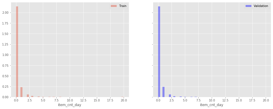
Target Distribution
fig, axes = plt.subplots(1, 2, figsize=(16,6), sharey=True)
sns.distplot(Y_train, kde=False, ax=axes[0], norm_hist=True, label='Train')
sns.distplot(Y_valid, kde=False, ax=axes[1], norm_hist=True, label='Validation', color='b')
axes[0].legend()
axes[1].legend();
First Level Models
Scaling and Encoding
Because we have encoded features related to the price and average features, it is important to have a common scale when feeding our dataset into models like the Linear Regression. These models are very sensitive to data scale
for col in tqdm_notebook(X_train.columns):
    if X_train[col].dtype!='int8' and X_train[col].dtype!='int16':
        scaler = MinMaxScaler().fit(X_train[[col]])

        X_train[col] = scaler.transform(X_train[[col]])
        X_valid[col] = scaler.transform(X_valid[[col]])
        X_valid_meta[col] = scaler.transform(X_valid_meta[[col]])
        X_test[col] = scaler.transform(X_test[[col]])
HBox(children=(IntProgress(value=0, max=72), HTML(value='')))
Simple Model Selection
In this section, we train several basic models with their default parameters and we compare how they perform on the validation set. The goal is to identify model with potential. The selected models will then be finely tuned.
Note: Our dataset contains categorical features encoded using index integers. In order to train a linear model on the dataset, we need to remove these categorical features from the sets.
# features to be removed when training a linear model
categorical_features = ['city_id', 'date_block_num', 'item_category_id',
                        'item_id', 'shop_id', 'subtype_id', 'type_id']
# select subset of features for linear models
X_train_lin = X_train[X_train.columns.difference(categorical_features)]
X_valid_lin = X_valid[X_valid.columns.difference(categorical_features)]
X_valid_meta_lin = X_valid_meta[X_valid_meta.columns.difference(categorical_features)]
X_test_lin = X_test[X_test.columns.difference(categorical_features)]
We now train several simple models using their default parameter to assess their potential.
Our candidates consist of a set of tree-based models and a set of models not able to handle categorical features. We therefore create a test and train set without categorical features.
models_trees = [ExtraTreesRegressor(n_jobs=-1, verbose=2),
                RandomForestRegressor(n_jobs=-1, verbose=2),
                LGBMRegressor(n_jobs=-1, verbose=2),
                XGBRegressor(n_jobs=-1, objective='reg:squarederror', verbose=2)]
models_lin = [Lasso(), ElasticNet(), BayesianRidge(), LinearRegression()]
# results summary
summary_cols = ['Model', 'Parameters (Pre)', 'train_RMSE', 'val_RMSE']
summary_df = pd.DataFrame(columns=summary_cols)

pred_valid_df = pd.DataFrame()
def train_estimator(x_train, y_train, x_valid, y_valid, estimators, df, pred_df):

    n_rows = df.shape[0]

    for idx, estimator in tqdm_notebook(enumerate(estimators)):

        # identify model
        df.loc[idx+n_rows, 'Model'] = estimator.__class__.__name__
        df.loc[idx+n_rows,'Parameters (Pre)'] = str(estimator.get_params())

        # train model
        print('-'*50)
        print("Training:", estimator.__class__.__name__)
        ts = time.time()
        estimator.fit(x_train, y_train)
        print('\ttraining time: {:.1f}s'.format(time.time()-ts))

        # compute metrics
        pred_valid = np.clip(estimator.predict(x_valid), 0., 20.)
        pred_train = np.clip(estimator.predict(x_train), 0., 20.)
        rmse_val = np.sqrt(mean_squared_error(y_valid, pred_valid))
        rmse_train = np.sqrt(mean_squared_error(y_train, pred_train))

        # save metrics
        df.loc[idx+n_rows, 'train_RMSE'] = rmse_train
        df.loc[idx+n_rows, 'val_RMSE'] = rmse_val

        pred_df[estimator.__class__.__name__] = pred_valid

        print(estimator.__class__.__name__, 'trained...')

        del estimator
        gc.collect()

    df = df.sort_values(['val_RMSE'])
    df.reset_index(drop=True)

    return df, pred_df
summary_df, pred_valid_df  = train_estimator(X_train_lin, Y_train,
                                             X_valid_lin, Y_valid,
                                             models_lin, summary_df, pred_valid_df)
HBox(children=(IntProgress(value=1, bar_style='info', max=1), HTML(value='')))


--------------------------------------------------
Training: Lasso
	training time: 6.5s
Lasso trained...
--------------------------------------------------
Training: ElasticNet
	training time: 4.4s
ElasticNet trained...
--------------------------------------------------
Training: BayesianRidge
	training time: 21.7s
BayesianRidge trained...
--------------------------------------------------
Training: LinearRegression
	training time: 7.9s
LinearRegression trained...
summary_df, pred_valid_df  = train_estimator(X_train, Y_train,
                             X_valid, Y_valid,
                             models_trees, summary_df, pred_valid_df)
HBox(children=(IntProgress(value=1, bar_style='info', max=1), HTML(value='')))


--------------------------------------------------
Training: ExtraTreesRegressor


[Parallel(n_jobs=-1)]: Using backend ThreadingBackend with 4 concurrent workers.


building tree 1 of 10building tree 2 of 10
building tree 3 of 10
building tree 4 of 10

building tree 5 of 10
building tree 6 of 10
building tree 7 of 10
building tree 8 of 10
building tree 9 of 10
building tree 10 of 10


[Parallel(n_jobs=-1)]: Done  10 out of  10 | elapsed:  9.8min finished


	training time: 591.2s


[Parallel(n_jobs=4)]: Using backend ThreadingBackend with 4 concurrent workers.
[Parallel(n_jobs=4)]: Done  10 out of  10 | elapsed:    1.6s finished
[Parallel(n_jobs=4)]: Using backend ThreadingBackend with 4 concurrent workers.
[Parallel(n_jobs=4)]: Done  10 out of  10 | elapsed:    7.8s finished


ExtraTreesRegressor trained...
--------------------------------------------------
Training: RandomForestRegressor


[Parallel(n_jobs=-1)]: Using backend ThreadingBackend with 4 concurrent workers.


building tree 1 of 10building tree 2 of 10
building tree 3 of 10
building tree 4 of 10

building tree 5 of 10
building tree 6 of 10
building tree 7 of 10
building tree 8 of 10
building tree 9 of 10
building tree 10 of 10


[Parallel(n_jobs=-1)]: Done  10 out of  10 | elapsed: 15.5min finished


	training time: 932.4s


[Parallel(n_jobs=4)]: Using backend ThreadingBackend with 4 concurrent workers.
[Parallel(n_jobs=4)]: Done  10 out of  10 | elapsed:    1.7s finished
[Parallel(n_jobs=4)]: Using backend ThreadingBackend with 4 concurrent workers.
[Parallel(n_jobs=4)]: Done  10 out of  10 | elapsed:    7.5s finished


RandomForestRegressor trained...
--------------------------------------------------
Training: LGBMRegressor
	training time: 64.9s
LGBMRegressor trained...
--------------------------------------------------
Training: XGBRegressor

	training time: 3223.7s
XGBRegressor trained...
Below are the results of our basic models. As we can see, the Lasso and ElasticNet model contain too much regularization and are not able to make predictions.
summary_df
| Model | Parameters (Pre) | train_RMSE | val_RMSE | |
|---|---|---|---|---|
| 6 | LGBMRegressor | {'boosting_type': 'gbdt', 'class_weight': None... | 0.826947 | 0.813052 |
| 7 | XGBRegressor | {'base_score': 0.5, 'booster': 'gbtree', 'cols... | 0.897198 | 0.822411 |
| 2 | BayesianRidge | {'alpha_1': 1e-06, 'alpha_2': 1e-06, 'compute_... | 0.933291 | 0.838651 |
| 3 | LinearRegression | {'copy_X': True, 'fit_intercept': True, 'n_job... | 0.933289 | 0.838666 |
| 5 | RandomForestRegressor | {'bootstrap': True, 'criterion': 'mse', 'max_d... | 0.329639 | 0.878088 |
| 4 | ExtraTreesRegressor | {'bootstrap': False, 'criterion': 'mse', 'max_... | 0 | 0.878273 |
| 0 | Lasso | {'alpha': 1.0, 'copy_X': True, 'fit_intercept'... | 1.21245 | 1.07186 |
| 1 | ElasticNet | {'alpha': 1.0, 'copy_X': True, 'fit_intercept'... | 1.21245 | 1.07186 |
# plot results
fig, ax = plt.subplots(figsize=(8,6))
g = sns.barplot("val_RMSE",
                "Model",
                data = summary_df)
g.set_xlabel("Mean Accuracy")
g = g.set_title("Validation scores")
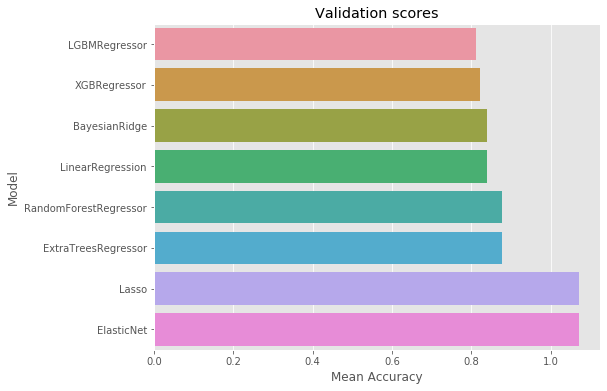
When blending models, we need to combine models that are not “too” correlated. Therefore, we plot the correlations in the predictions of our models.
# Compute the correlation matrix
corr = pred_valid_df.corr()

# Generate a mask for the upper triangle
mask = np.zeros_like(corr, dtype=np.bool)
mask[np.triu_indices_from(mask)] = True

# Generate a custom diverging colormap
cmap = sns.diverging_palette(220, 10, as_cmap=True)

with sns.axes_style("white"):
    # Set up the matplotlib figure
    f, ax = plt.subplots(figsize=(12, 12))

    # Draw the heatmap with the mask and correct aspect ratio
    sns.heatmap(corr, mask=mask, cmap=cmap, vmax=1.0,vmin=0.0, center=1/2.,annot=True,
                square=True, linewidths=.5, cbar_kws={"shrink": .4})

    ax.set_ylim((8,0));
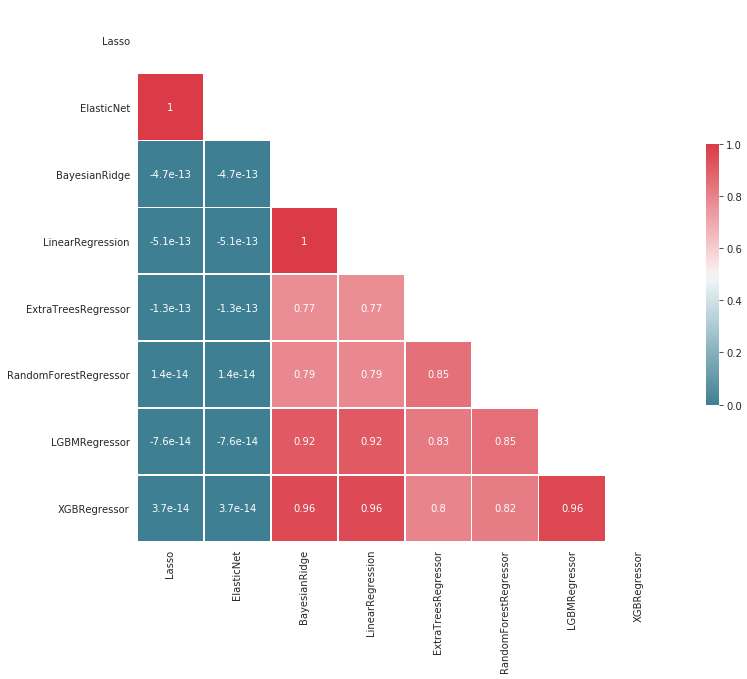
As we can see, the Lasso and ElasticNet model only predict 0, this is due to a poor regularization parameter value. We will keep these model and finely tune them
def tune_model(estimator, X_train, Y_train, X_val, Y_val, grid_params):
    # extract parameters to be tuned and candidate values
    params = grid_params.keys()
    values = grid_params.values()

    # create all combinations
    combinations = product(*values)

    # store results
    scores = []
    return_obj = {}
    parameters = []

    # iterate
    for idx, combo in enumerate(combinations):
        # format header for readability
        print('-'*50)
        print("MODEL {0}".format(idx))

        ts = time.time()

        # recreate input params
        current_param = dict(zip(params, combo))
        print(current_param)
        parameters.append(current_param)

        # train model
        model = estimator(**current_param)
        model.fit(X_train, Y_train)
        print('\ttraining done: {:.2f}s'.format(time.time()-ts))

        # make predictions
        pred_validaiton = model.predict(X_val)

        # compute metrics
        mse = mean_squared_error(Y_val, pred_validaiton)
        rmse = np.sqrt(mse)
        print('RMSE SCORE: {:.5f}'.format(rmse))

        # save scores
        scores.append(rmse)

        # checkpoint
        best_score = np.min(scores)
        print('Best score: {:.5f}'.format(best_score))
        best_model = parameters[np.argmin(scores)]
        print('Best model: {}'.format(best_model))

        del best_score
        del best_model
        del pred_validaiton
        del model
        gc.collect

    # scores and models
    print('-'*50)
    print('SUMMARY')
    scores = np.array(scores)
    best_score = np.min(scores)
    best_model = parameters[np.argmin(scores)]
    print('Best score: {:.5f}'.format(best_score))
    print('Best model: {}'.format(best_model))

    return_obj['scores'] = scores
    return_obj['best_score'] = best_score
    return_obj['best_model_params'] = best_model

    return return_obj
Ridge Regression
alphas = [265, 270, 275]
grid_params = {'alpha':alphas}
val_res = tune_model(Ridge, X_train_lin, Y_train,
                   X_valid_lin, Y_valid, grid_params)
--------------------------------------------------
MODEL 0
{'alpha': 265}
	training done: 10.59s
RMSE SCORE: 0.83796
Best score: 0.83796
Best model: {'alpha': 265}
--------------------------------------------------
MODEL 1
{'alpha': 270}
	training done: 3.67s
RMSE SCORE: 0.83796
Best score: 0.83796
Best model: {'alpha': 270}
--------------------------------------------------
MODEL 2
{'alpha': 275}
	training done: 2.75s
RMSE SCORE: 0.83796
Best score: 0.83796
Best model: {'alpha': 270}
--------------------------------------------------
SUMMARY
Best score: 0.83796
Best model: {'alpha': 270}
Lasso
alphas = 10**np.linspace(-4.2, -3.6, 5)
grid_params = {'alpha':alphas}
val_res = tune_model(Lasso, X_train_lin, Y_train,
                   X_valid_lin, Y_valid, grid_params)
--------------------------------------------------
MODEL 0
{'alpha': 6.309573444801929e-05}
	training done: 158.73s
RMSE SCORE: 0.83807
Best score: 0.83807
Best model: {'alpha': 6.309573444801929e-05}
--------------------------------------------------
MODEL 1
{'alpha': 8.912509381337459e-05}
	training done: 129.75s
RMSE SCORE: 0.83810
Best score: 0.83807
Best model: {'alpha': 6.309573444801929e-05}
--------------------------------------------------
MODEL 2
{'alpha': 0.0001258925411794166}
	training done: 49.31s
RMSE SCORE: 0.83808
Best score: 0.83807
Best model: {'alpha': 6.309573444801929e-05}
--------------------------------------------------
MODEL 3
{'alpha': 0.00017782794100389227}
	training done: 52.77s
RMSE SCORE: 0.83824
Best score: 0.83807
Best model: {'alpha': 6.309573444801929e-05}
--------------------------------------------------
MODEL 4
{'alpha': 0.00025118864315095795}
	training done: 52.73s
RMSE SCORE: 0.83879
Best score: 0.83807
Best model: {'alpha': 6.309573444801929e-05}
--------------------------------------------------
SUMMARY
Best score: 0.83807
Best model: {'alpha': 6.309573444801929e-05}
Bayesian Ridge
br_alpha_1 = 10**np.linspace(+4,+6,5)
br_alpha_2 = 10**np.linspace(-8,-6,5)
br_lambda_1 = 10**np.linspace(+4,+6,5)
br_lambda_2 = 10**np.linspace(+1,+3,5)

grid_params = {'alpha_1': br_alpha_1, 'alpha_2': br_alpha_2,
               'lambda_1': br_lambda_1, 'lambda_2': br_lambda_2}
val_res = tune_model(BayesianRidge, X_train_lin, Y_train,
                    X_valid_lin, Y_valid, grid_params)
--------------------------------------------------
MODEL 0
{'alpha_1': 10000.0, 'alpha_2': 1e-08, 'lambda_1': 10000.0, 'lambda_2': 10.0}
	training done: 29.31s
RMSE SCORE: 0.83807
Best score: 0.83807
Best model: {'alpha_1': 10000.0, 'alpha_2': 1e-08, 'lambda_1': 10000.0, 'lambda_2': 10.0}
--------------------------------------------------
MODEL 1
{'alpha_1': 10000.0, 'alpha_2': 1e-08, 'lambda_1': 10000.0, 'lambda_2': 31.622776601683793}
	training done: 16.63s
RMSE SCORE: 0.83815
Best score: 0.83807
Best model: {'alpha_1': 10000.0, 'alpha_2': 1e-08, 'lambda_1': 10000.0, 'lambda_2': 10.0}
--------------------------------------------------
MODEL 2
{'alpha_1': 10000.0, 'alpha_2': 1e-08, 'lambda_1': 10000.0, 'lambda_2': 100.0}
	training done: 16.15s
RMSE SCORE: 0.83832
Best score: 0.83807
Best model: {'alpha_1': 10000.0, 'alpha_2': 1e-08, 'lambda_1': 10000.0, 'lambda_2': 10.0}
--------------------------------------------------
MODEL 3
{'alpha_1': 10000.0, 'alpha_2': 1e-08, 'lambda_1': 10000.0, 'lambda_2': 316.22776601683796}
	training done: 16.43s
RMSE SCORE: 0.83852
Best score: 0.83807
Best model: {'alpha_1': 10000.0, 'alpha_2': 1e-08, 'lambda_1': 10000.0, 'lambda_2': 10.0}
...
--------------------------------------------------
MODEL 624
{'alpha_1': 1000000.0, 'alpha_2': 1e-06, 'lambda_1': 1000000.0, 'lambda_2': 1000.0}
	training done: 15.20s
RMSE SCORE: 0.83822
Best score: 0.83796
Best model: {'alpha_1': 10000.0, 'alpha_2': 1e-07, 'lambda_1': 316227.7660168379, 'lambda_2': 1000.0}
--------------------------------------------------
SUMMARY
Best score: 0.83796
Best model: {'alpha_1': 10000.0, 'alpha_2': 1e-07, 'lambda_1': 316227.7660168379, 'lambda_2': 1000.0}
Random Forest
grid_params={'max_depth': [10, 20, 30, None],
             'max_features': ['auto', 'sqrt'],
             'min_samples_split': [5, 10],
             'n_estimators': [10, 50, 100],
             'n_jobs':[-1]}

val_res = tune_model(RandomForestRegressor, X_train, Y_train,
                    X_valid, Y_valid, grid_params)
--------------------------------------------------
MODEL 0
{'max_depth': 10, 'max_features': 'auto', 'min_samples_split': 5, 'n_estimators': 10, 'n_jobs': -1}
	training done: 546.59s
RMSE SCORE: 0.82886
Best score: 0.82886
Best model: {'max_depth': 10, 'max_features': 'auto', 'min_samples_split': 5, 'n_estimators': 10, 'n_jobs': -1}
--------------------------------------------------
MODEL 1
{'max_depth': 10, 'max_features': 'auto', 'min_samples_split': 5, 'n_estimators': 50, 'n_jobs': -1}
	training done: 2117.12s
RMSE SCORE: 0.82208
Best score: 0.82208
Best model: {'max_depth': 10, 'max_features': 'auto', 'min_samples_split': 5, 'n_estimators': 50, 'n_jobs': -1}
--------------------------------------------------
MODEL 2
{'max_depth': 10, 'max_features': 'auto', 'min_samples_split': 5, 'n_estimators': 100, 'n_jobs': -1}
	training done: 4011.42s
RMSE SCORE: 0.82328
Best score: 0.82208
Best model: {'max_depth': 10, 'max_features': 'auto', 'min_samples_split': 5, 'n_estimators': 50, 'n_jobs': -1}
...
--------------------------------------------------
MODEL 47
{'max_depth': None, 'max_features': 'sqrt', 'min_samples_split': 10, 'n_estimators': 100, 'n_jobs': -1}
	training done: 1189.53s
RMSE SCORE: 0.82544
Best score: 0.80872
Best model: {'max_depth': 20, 'max_features': 'sqrt', 'min_samples_split': 10, 'n_estimators': 100, 'n_jobs': -1}
--------------------------------------------------
SUMMARY
Best score: 0.80872
Best model: {'max_depth': 20, 'max_features': 'sqrt', 'min_samples_split': 10, 'n_estimators': 100, 'n_jobs': -1}
grid_params={'max_depth': [10],
             'max_features': ['auto'],
             'min_samples_split': [5],
             'n_estimators': [500],
             'n_jobs':[-1],
             'verbose':[1]}

val_res = tune_model(RandomForestRegressor, X_train, Y_train,
                    X_valid, Y_valid, grid_params)
--------------------------------------------------
MODEL 0
{'max_depth': 10, 'max_features': 'auto', 'min_samples_split': 5, 'n_estimators': 500, 'n_jobs': -1, 'verbose': 1}


[Parallel(n_jobs=-1)]: Using backend ThreadingBackend with 4 concurrent workers.
[Parallel(n_jobs=-1)]: Done  42 tasks      | elapsed: 30.1min
[Parallel(n_jobs=-1)]: Done 192 tasks      | elapsed: 113.6min
[Parallel(n_jobs=-1)]: Done 442 tasks      | elapsed: 255.3min
[Parallel(n_jobs=-1)]: Done 500 out of 500 | elapsed: 287.2min finished


	training done: 17241.45s


[Parallel(n_jobs=4)]: Using backend ThreadingBackend with 4 concurrent workers.
[Parallel(n_jobs=4)]: Done  42 tasks      | elapsed:    0.9s
[Parallel(n_jobs=4)]: Done 192 tasks      | elapsed:    4.9s
[Parallel(n_jobs=4)]: Done 442 tasks      | elapsed:   10.2s


RMSE SCORE: 0.82104
Best score: 0.82104
Best model: {'max_depth': 10, 'max_features': 'auto', 'min_samples_split': 5, 'n_estimators': 500, 'n_jobs': -1, 'verbose': 1}
--------------------------------------------------
SUMMARY
Best score: 0.82104
Best model: {'max_depth': 10, 'max_features': 'auto', 'min_samples_split': 5, 'n_estimators': 500, 'n_jobs': -1, 'verbose': 1}


[Parallel(n_jobs=4)]: Done 500 out of 500 | elapsed:   11.4s finished
LightGBM
def tune_model_lgb(lgb_train_, lgb_valid_, grid_params):
    # extract parameters to be tuned and candidate values
    params = grid_params.keys()
    values = grid_params.values()

    # create all combinations
    combinations = product(*values)

    # store results
    scores = []
    return_obj = {}
    parameters = []

    # iterate
    for idx, combo in enumerate(combinations):
        # format header for readability
        print('-'*50)
        print("MODEL {0}".format(idx))

        ts = time.time()

        # recreate input params
        current_param = dict(zip(params, combo))
        print(current_param)
        parameters.append(current_param)

        # train model
        gbm = lgb.train(current_param,
                lgb_train,
                num_boost_round=300,
                valid_sets=lgb_valid,
                early_stopping_rounds=5)

        print('\ttraining done: {:.2f}s'.format(time.time()-ts))

        # make predictions
        y_pred = np.clip(gbm.predict(X_valid, num_iteration=gbm.best_iteration),0.,20.)

        # compute metrics
        mse = mean_squared_error(Y_valid, y_pred)
        rmse = np.sqrt(mse)
        print('RMSE SCORE: {:.5f}'.format(rmse))

        # save scores
        scores.append(rmse)

        # checkpoint
        best_score = np.min(scores)
        print('Best score: {:.5f}'.format(best_score))
        best_model = parameters[np.argmin(scores)]
        print('Best model: {}'.format(best_model))

        del best_score
        del best_model
        del y_pred
        del gbm
        gc.collect

    # scores and models
    print('-'*50)
    print('SUMMARY')
    scores = np.array(scores)
    best_score = np.min(scores)
    best_model = parameters[np.argmin(scores)]
    print('Best score: {:.5f}'.format(best_score))
    print('Best model: {}'.format(best_model))

    return_obj['scores'] = scores
    return_obj['best_score'] = best_score
    return_obj['best_model_params'] = best_model

    return return_obj
# isolate categorical features
indexes_of_categories = [X_train.columns.get_loc(col) for col in categorical_features]
# create lbg training and validation set
lgb_train = lgb.Dataset(data=X_train, label=Y_train, categorical_feature=indexes_of_categories, free_raw_data=False)
lgb_valid = lgb.Dataset(data=X_valid, label=Y_valid, categorical_feature=indexes_of_categories, free_raw_data=False)

params_gs = {
    'num_leaves': [17,31,51],
    'min_data_in_leaf':[10,20,30],
    'max_depth':[-1,10],
    'learning_rate': [0.05,0.1],
    'feature_fraction':[0.5, 0.6, 0.7,0.8,0.9],
    'bagging_fraction':[0.5,0.7,0.8],
    'max_bin':[255],
    'boosting_type': ['gbdt'],
    'objective': ['regression'],
    'metric': ['l2'],
    'bagging_freq': [5,6,7],
    'verbose': [-1]
}

light_gbm = tune_model_lgb(lgb_train, lgb_valid, params_gs)
--------------------------------------------------
MODEL 0
{'num_leaves': 17, 'min_data_in_leaf': 10, 'max_depth': -1, 'learning_rate': 0.05, 'feature_fraction': 0.5, 'bagging_fraction': 0.5, 'max_bin': 255, 'boosting_type': 'gbdt', 'objective': 'regression', 'metric': 'l2', 'bagging_freq': 5, 'verbose': -1}


[1]	valid_0's l2: 1.10527
Training until validation scores don't improve for 5 rounds
[2]	valid_0's l2: 1.07531
[3]	valid_0's l2: 1.05201
[4]	valid_0's l2: 1.02279
[5]	valid_0's l2: 0.998551
[6]	valid_0's l2: 0.974025
[7]	valid_0's l2: 0.952692
[8]	valid_0's l2: 0.932333
[9]	valid_0's l2: 0.91344
[10]	valid_0's l2: 0.895566
[11]	valid_0's l2: 0.876383
[12]	valid_0's l2: 0.862929
[13]	valid_0's l2: 0.850901
[14]	valid_0's l2: 0.838443
[15]	valid_0's l2: 0.823629
[16]	valid_0's l2: 0.815305
[17]	valid_0's l2: 0.803962
[18]	valid_0's l2: 0.798741
[19]	valid_0's l2: 0.791434
[20]	valid_0's l2: 0.783215
[21]	valid_0's l2: 0.776634
[22]	valid_0's l2: 0.768956
[23]	valid_0's l2: 0.764029
[24]	valid_0's l2: 0.757802
[25]	valid_0's l2: 0.754147
[26]	valid_0's l2: 0.749015
[27]	valid_0's l2: 0.743662
[28]	valid_0's l2: 0.738082
[29]	valid_0's l2: 0.735406
[30]	valid_0's l2: 0.731135
[31]	valid_0's l2: 0.72884
[32]	valid_0's l2: 0.727529
[33]	valid_0's l2: 0.724651
[34]	valid_0's l2: 0.72392
[35]	valid_0's l2: 0.720609
[36]	valid_0's l2: 0.720633
[37]	valid_0's l2: 0.719136
[38]	valid_0's l2: 0.716923
[39]	valid_0's l2: 0.714208
[40]	valid_0's l2: 0.712108
[41]	valid_0's l2: 0.710699
[42]	valid_0's l2: 0.710426
[43]	valid_0's l2: 0.709536
[44]	valid_0's l2: 0.710491
[45]	valid_0's l2: 0.707844
[46]	valid_0's l2: 0.706848
[47]	valid_0's l2: 0.705889
[48]	valid_0's l2: 0.703528
[49]	valid_0's l2: 0.701249
[50]	valid_0's l2: 0.701599
[51]	valid_0's l2: 0.700817
[52]	valid_0's l2: 0.700734
[53]	valid_0's l2: 0.699862
[54]	valid_0's l2: 0.699969
[55]	valid_0's l2: 0.699991
[56]	valid_0's l2: 0.699688
[57]	valid_0's l2: 0.699316
[58]	valid_0's l2: 0.697707
[59]	valid_0's l2: 0.697867
[60]	valid_0's l2: 0.697003
[61]	valid_0's l2: 0.695797
[62]	valid_0's l2: 0.694803
[63]	valid_0's l2: 0.694291
[64]	valid_0's l2: 0.693099
[65]	valid_0's l2: 0.692775
[66]	valid_0's l2: 0.693045
[67]	valid_0's l2: 0.691834
[68]	valid_0's l2: 0.692186
[69]	valid_0's l2: 0.692687
[70]	valid_0's l2: 0.692229
[71]	valid_0's l2: 0.692593
[72]	valid_0's l2: 0.692336
Early stopping, best iteration is:
[67]	valid_0's l2: 0.691834
	training done: 40.75s
RMSE SCORE: 0.83516
Best score: 0.83516
Best model: {'num_leaves': 17, 'min_data_in_leaf': 10, 'max_depth': -1, 'learning_rate': 0.05, 'feature_fraction': 0.5, 'bagging_fraction': 0.5, 'max_bin': 255, 'boosting_type': 'gbdt', 'objective': 'regression', 'metric': 'l2', 'bagging_freq': 5, 'verbose': -1}
--------------------------------------------------
MODEL 1
{'num_leaves': 17, 'min_data_in_leaf': 10, 'max_depth': -1, 'learning_rate': 0.05, 'feature_fraction': 0.5, 'bagging_fraction': 0.5, 'max_bin': 255, 'boosting_type': 'gbdt', 'objective': 'regression', 'metric': 'l2', 'bagging_freq': 6, 'verbose': -1}


[1]	valid_0's l2: 1.10527
Training until validation scores don't improve for 5 rounds
[2]	valid_0's l2: 1.07531
[3]	valid_0's l2: 1.05201
[4]	valid_0's l2: 1.02279
[5]	valid_0's l2: 0.998551
[6]	valid_0's l2: 0.97405
[7]	valid_0's l2: 0.95349
[8]	valid_0's l2: 0.932658
[9]	valid_0's l2: 0.914223
[10]	valid_0's l2: 0.897632
[11]	valid_0's l2: 0.877349
[12]	valid_0's l2: 0.863744
[13]	valid_0's l2: 0.851036
[14]	valid_0's l2: 0.838301
[15]	valid_0's l2: 0.823764
[16]	valid_0's l2: 0.816064
[17]	valid_0's l2: 0.805195
[18]	valid_0's l2: 0.79905
[19]	valid_0's l2: 0.791872
[20]	valid_0's l2: 0.783252
[21]	valid_0's l2: 0.777125
[22]	valid_0's l2: 0.76982
[23]	valid_0's l2: 0.765262
[24]	valid_0's l2: 0.759256
[25]	valid_0's l2: 0.75549
[26]	valid_0's l2: 0.750393
[27]	valid_0's l2: 0.744901
[28]	valid_0's l2: 0.739169
[29]	valid_0's l2: 0.736655
[30]	valid_0's l2: 0.732419
[31]	valid_0's l2: 0.730543
[32]	valid_0's l2: 0.72918
[33]	valid_0's l2: 0.725655
[34]	valid_0's l2: 0.725163
[35]	valid_0's l2: 0.721856
[36]	valid_0's l2: 0.721893
[37]	valid_0's l2: 0.720522
[38]	valid_0's l2: 0.717873
[39]	valid_0's l2: 0.714776
[40]	valid_0's l2: 0.712635
[41]	valid_0's l2: 0.710812
[42]	valid_0's l2: 0.710365
[43]	valid_0's l2: 0.70942
[44]	valid_0's l2: 0.709538
[45]	valid_0's l2: 0.707223
[46]	valid_0's l2: 0.705169
[47]	valid_0's l2: 0.703678
[48]	valid_0's l2: 0.701343
[49]	valid_0's l2: 0.700215
[50]	valid_0's l2: 0.700314
[51]	valid_0's l2: 0.699423
[52]	valid_0's l2: 0.699303
[53]	valid_0's l2: 0.697868
[54]	valid_0's l2: 0.697933
[55]	valid_0's l2: 0.697991
[56]	valid_0's l2: 0.698016
[57]	valid_0's l2: 0.697487
[58]	valid_0's l2: 0.696206
[59]	valid_0's l2: 0.69619
[60]	valid_0's l2: 0.695404
[61]	valid_0's l2: 0.694171
[62]	valid_0's l2: 0.693438
[63]	valid_0's l2: 0.693584
[64]	valid_0's l2: 0.692399
[65]	valid_0's l2: 0.691994
[66]	valid_0's l2: 0.692421
[67]	valid_0's l2: 0.691399
[68]	valid_0's l2: 0.691757
[69]	valid_0's l2: 0.692146
[70]	valid_0's l2: 0.691961
[71]	valid_0's l2: 0.69215
[72]	valid_0's l2: 0.692097
Early stopping, best iteration is:
[67]	valid_0's l2: 0.691399
	training done: 21.72s
RMSE SCORE: 0.83113
Best score: 0.83113
Best model: {'num_leaves': 17, 'min_data_in_leaf': 10, 'max_depth': -1, 'learning_rate': 0.05, 'feature_fraction': 0.5, 'bagging_fraction': 0.5, 'max_bin': 255, 'boosting_type': 'gbdt', 'objective': 'regression', 'metric': 'l2', 'bagging_freq': 6, 'verbose': -1}

--------------------------------------------------
MODEL 1619
{'num_leaves': 51, 'min_data_in_leaf': 30, 'max_depth': 10, 'learning_rate': 0.1, 'feature_fraction': 0.9, 'bagging_fraction': 0.8, 'max_bin': 255, 'boosting_type': 'gbdt', 'objective': 'regression', 'metric': 'l2', 'bagging_freq': 7, 'verbose': -1}


[1]	valid_0's l2: 1.07129
Training until validation scores don't improve for 5 rounds
[2]	valid_0's l2: 1.00838
[3]	valid_0's l2: 0.962023
[4]	valid_0's l2: 0.919852
[5]	valid_0's l2: 0.887095
[6]	valid_0's l2: 0.851199
[7]	valid_0's l2: 0.831776
[8]	valid_0's l2: 0.814751
[9]	valid_0's l2: 0.800856
[10]	valid_0's l2: 0.789847
[11]	valid_0's l2: 0.780962
[12]	valid_0's l2: 0.774846
[13]	valid_0's l2: 0.769069
[14]	valid_0's l2: 0.764315
[15]	valid_0's l2: 0.753459
[16]	valid_0's l2: 0.749205
[17]	valid_0's l2: 0.747357
[18]	valid_0's l2: 0.744728
[19]	valid_0's l2: 0.744139
[20]	valid_0's l2: 0.744054
[21]	valid_0's l2: 0.742659
[22]	valid_0's l2: 0.743116
[23]	valid_0's l2: 0.743458
[24]	valid_0's l2: 0.73827
[25]	valid_0's l2: 0.738553
[26]	valid_0's l2: 0.733934
[27]	valid_0's l2: 0.734115
[28]	valid_0's l2: 0.734221
[29]	valid_0's l2: 0.734035
[30]	valid_0's l2: 0.733784
[31]	valid_0's l2: 0.734618
[32]	valid_0's l2: 0.7356
[33]	valid_0's l2: 0.733096
[34]	valid_0's l2: 0.732815
[35]	valid_0's l2: 0.733961
[36]	valid_0's l2: 0.735807
[37]	valid_0's l2: 0.735931
[38]	valid_0's l2: 0.735966
[39]	valid_0's l2: 0.736026
Early stopping, best iteration is:
[34]	valid_0's l2: 0.732815
	training done: 25.08s
RMSE SCORE: 0.86025
Best score: 0.82441
Best model: {'num_leaves': 51, 'min_data_in_leaf': 30, 'max_depth': 10, 'learning_rate': 0.05, 'feature_fraction': 0.5, 'bagging_fraction': 0.5, 'max_bin': 255, 'boosting_type': 'gbdt', 'objective': 'regression', 'metric': 'l2', 'bagging_freq': 5, 'verbose': -1}
--------------------------------------------------
SUMMARY
Best score: 0.82441
Best model: {'num_leaves': 51, 'min_data_in_leaf': 30, 'max_depth': 10, 'learning_rate': 0.05, 'feature_fraction': 0.5, 'bagging_fraction': 0.5, 'max_bin': 255, 'boosting_type': 'gbdt', 'objective': 'regression', 'metric': 'l2', 'bagging_freq': 5, 'verbose': -1}
XGBoost
best_params = {'learning_rate': 0.16, 'n_estimators': 500,
               'max_depth': 6, 'min_child_weight': 7,
               'subsample': 0.9, 'colsample_bytree': 0.7, 'nthread': -1,
               'scale_pos_weight': 1, 'random_state': 42, 'verbose':2}

model = XGBRegressor(**best_params)
model.fit(X_train, Y_train, eval_metric="rmse", eval_set=[(X_valid, Y_valid)],
          verbose=True,early_stopping_rounds = 50)
[0]	validation_0-rmse:1.03205
Will train until validation_0-rmse hasn't improved in 50 rounds.
[1]	validation_0-rmse:0.980421
[2]	validation_0-rmse:0.94645
[3]	validation_0-rmse:0.913994
[4]	validation_0-rmse:0.891504
[5]	validation_0-rmse:0.874951
[6]	validation_0-rmse:0.862584
[7]	validation_0-rmse:0.853669
[8]	validation_0-rmse:0.847595
[9]	validation_0-rmse:0.839851
[10]	validation_0-rmse:0.837036
[11]	validation_0-rmse:0.834322
[12]	validation_0-rmse:0.83262
[13]	validation_0-rmse:0.83206
[14]	validation_0-rmse:0.830011
[15]	validation_0-rmse:0.828429
[16]	validation_0-rmse:0.827463
[17]	validation_0-rmse:0.826978
[18]	validation_0-rmse:0.825869
[19]	validation_0-rmse:0.824109
[20]	validation_0-rmse:0.823856
[21]	validation_0-rmse:0.823428
[22]	validation_0-rmse:0.822876
[23]	validation_0-rmse:0.821865
[24]	validation_0-rmse:0.821441
[25]	validation_0-rmse:0.821135
[26]	validation_0-rmse:0.820952
[27]	validation_0-rmse:0.820293
[28]	validation_0-rmse:0.819232
[29]	validation_0-rmse:0.821048
[30]	validation_0-rmse:0.821688
[31]	validation_0-rmse:0.82166
[32]	validation_0-rmse:0.82134
[33]	validation_0-rmse:0.821112
[34]	validation_0-rmse:0.82101
[35]	validation_0-rmse:0.82121
[36]	validation_0-rmse:0.821139
[37]	validation_0-rmse:0.821079
[38]	validation_0-rmse:0.82094
[39]	validation_0-rmse:0.821209
[40]	validation_0-rmse:0.820822
[41]	validation_0-rmse:0.821023
[42]	validation_0-rmse:0.820533
[43]	validation_0-rmse:0.820379
[44]	validation_0-rmse:0.819605
[45]	validation_0-rmse:0.819557
[46]	validation_0-rmse:0.819411
[47]	validation_0-rmse:0.819752
[48]	validation_0-rmse:0.820246
[49]	validation_0-rmse:0.820295
[50]	validation_0-rmse:0.820421
[51]	validation_0-rmse:0.820169
[52]	validation_0-rmse:0.819825
[53]	validation_0-rmse:0.819881
[54]	validation_0-rmse:0.819917
[55]	validation_0-rmse:0.819968
[56] . . .
[124]	validation_0-rmse:0.820778
[125]	validation_0-rmse:0.82067
[126]	validation_0-rmse:0.82077
[127]	validation_0-rmse:0.820908
[128]	validation_0-rmse:0.821074
[129]	validation_0-rmse:0.821126
[130]	validation_0-rmse:0.821155
[131]	validation_0-rmse:0.821098
[132]	validation_0-rmse:0.821102
[133]	validation_0-rmse:0.821045
[134]	validation_0-rmse:0.821084
[135]	validation_0-rmse:0.821045
[136]	validation_0-rmse:0.820932
[137]	validation_0-rmse:0.820839
[138]	validation_0-rmse:0.820851
[139]	validation_0-rmse:0.821082
[140]	validation_0-rmse:0.820964
[141]	validation_0-rmse:0.820966
[142]	validation_0-rmse:0.820985
[143]	validation_0-rmse:0.821103
[144]	validation_0-rmse:0.821175
[145]	validation_0-rmse:0.820316
[146]	validation_0-rmse:0.820125
[147]	validation_0-rmse:0.82009
[148]	validation_0-rmse:0.819621
Stopping. Best iteration:
[98]	validation_0-rmse:0.818906


XGBRegressor(base_score=0.5, booster='gbtree', colsample_bylevel=1,
             colsample_bynode=1, colsample_bytree=0.7, gamma=0,
             importance_type='gain', learning_rate=0.16, max_delta_step=0,
             max_depth=6, min_child_weight=7, missing=None, n_estimators=500,
             n_jobs=1, nthread=-1, objective='reg:linear', random_state=42,
             reg_alpha=0, reg_lambda=1, scale_pos_weight=1, seed=None,
             silent=None, subsample=0.9, verbose=2, verbosity=1)
Final Models
Based on the above tuned models, we finally trained the models on months 12 to 27, then we make predictions for months 28 to 34. We then stack the models and trained the stacked model using months 28 to 33. Finally, we make predictions on month 34. Here are the summaries of our tuning process:
Step 1: Model training
# combine the X_train and X_train_valid dataframes
all_data = X_train.append(X_valid)
all_target = Y_train.append(Y_valid)

all_data_lin = X_train_lin.append(X_valid_lin)
all_dates = X_train_dates.append(X_valid_dates)
# we create 2nd level feeature matrix, init it with zeros first
X_train_valid_level2 = np.zeros([X_valid_dates.shape[0], 6])
X_test_level2 = np.zeros([X_valid_meta_dates.shape[0], 6])
X_submit = np.zeros([X_test.shape[0], 6])

# Now fill `X_train_valid_level2` with metafeatures
for cur_block_num in [28, 29, 30, 31, 32]:

    print("Testing on month: {}".format(cur_block_num))

    '''
        1. Split `X_train` into parts
           Remember, that corresponding dates are stored in `dates_train`
        2. Fit Ridge Regression
        3. Fit Lasso Regression
        4. Fit Bayesian Ridge
        5. Fit Random Forest
        6. Fit LightGBM
        7. Fit XGB
        8. Store predictions from 2. to 7. in the right place of `X_train_valid_level2`.
           You can use `dates_train_level2` for it
           Make sure the order of the meta-features is the same as in `X_test_level2`
    '''

    # 1. Split `X_train` into parts
    # first chunk from month 1 to month cur_block_num-1 (for training)
    # secondd chunk for month cur_block_num (test)
    X_train_temp = all_data.loc[all_dates <  cur_block_num]
    X_train_lin_temp = all_data_lin.loc[all_dates <  cur_block_num]

    X_test_temp =  all_data.loc[all_dates == cur_block_num]
    X_test_lin_temp = all_data_lin.loc[all_dates ==  cur_block_num]

    y_train_temp = all_target.loc[all_dates <  cur_block_num].values
    y_test_temp = all_target.loc[all_dates == cur_block_num].values

    # 2. Fit Ridge Regression
    model = Ridge(alpha=270)
    model.fit(X_train_lin_temp.values, y_train_temp)

    # predict level2
    pred_ridge = model.predict(X_test_lin_temp.values)
    # predict month 33
    pred_ridge_33 = model.predict(X_valid_meta_lin)
    # predict month 34
    pred_ridge_34 = model.predict(X_test_lin)
    print('\t done with Ridge')

    # 3. Fit Lasso Regression
    model = Lasso(alpha=6.309573444801929e-05)
    model.fit(X_train_lin_temp.values, y_train_temp)
    # predict level 2
    pred_lasso = model.predict(X_test_lin_temp.values)
    # predict month 33
    pred_lasso_33 = model.predict(X_valid_meta_lin)
    # predict month 34
    pred_lasso_34 = model.predict(X_test_lin)
    print('\t done with Lasso')

    # 4. Fit Bayesian Ridge
    model = BayesianRidge(
        alpha_1=10000.0, alpha_2=1e-07,
        lambda_1=316227.7660168379,lambda_2=1000.0
    )
    model.fit(X_train_lin_temp.values, y_train_temp)
    # predict level 2
    pred_bayesian = model.predict(X_test_lin_temp.values)
    # predict month 33
    pred_bayesian_33 = model.predict(X_valid_meta_lin)
    # predict month 34
    pred_bayesian_34 = model.predict(X_test_lin)
    print('\t done with Bayesian')

    # 5. Fit Random Forest
    model = RandomForestRegressor(
        max_depth=20, max_features='sqrt',
        min_samples_split=10, n_estimators=100, n_jobs=-1)
    model.fit(X_train_temp, y_train_temp)
    # predict level 2
    pred_rdm = model.predict(X_test_temp.values)
    # predict month 33
    pred_rdm_33 = model.predict(X_valid_meta)
    # predict month 34
    pred_rdm_34 = model.predict(X_test)
    print('\t done with Random Forest')

    # 6. Fit LightGBM
    # create lbg training and validation set
    lgb_train = lgb.Dataset(
        data=X_train_temp, label=y_train_temp,
        categorical_feature=indexes_of_categories,
        free_raw_data=False
    )

    params = {
        'num_leaves': 51, 'min_data_in_leaf': 30,
        'max_depth': 10, 'learning_rate': 0.05,
        'feature_fraction': 0.5, 'bagging_fraction': 0.5,
        'max_bin': 255, 'boosting_type': 'gbdt',
        'objective': 'regression', 'metric': 'l2',
        'bagging_freq': 5, 'verbose': -1}

    model = lgb.train(params,
                lgb_train,
                num_boost_round=300)
    # predict level 2
    pred_lgb = model.predict(X_test_temp)
    # predict month 33
    pred_lgb_33 = model.predict(X_valid_meta)
    # predict month 34
    pred_lgb_34 = model.predict(X_test)
    print('\t done with LGBM')

    # 7. Fit XGBoost
    model = XGBRegressor(
        learning_rate=0.16, n_estimators=500,
        max_depth=6, min_child_weight=7,
        subsample=0.9, colsample_bytree=0.7,
        nthread=-1, scale_pos_weight=1, random_state=42,
        verbose=0,
    )
    model.fit(X_train_temp, y_train_temp, eval_metric="rmse", eval_set=[(X_test_temp, y_test_temp)],
          verbose=False,early_stopping_rounds = 50)
    # predict level 2
    pred_xgb = model.predict(X_test_temp)
    # predict month 33
    pred_xgb_33 = model.predict(X_valid_meta)
    # predict month 34
    pred_xgb_34 = model.predict(X_test)
    print('\t done with XGB')

    # 8. Store predictions from 2. to 7. in the right place of `X_train_valid_level2`.
    # You can use `dates_train_level2` for it
    indexes = X_valid_dates.index[X_valid_dates == cur_block_num]
    indexes_shift = X_valid_dates.index.min()
    indexes = indexes - indexes_shift

    X_train_valid_level2[indexes, 0] = pred_ridge
    X_train_valid_level2[indexes, 1] = pred_lasso
    X_train_valid_level2[indexes, 2] = pred_bayesian
    X_train_valid_level2[indexes, 3] = pred_rdm
    X_train_valid_level2[indexes, 4] = pred_lgb
    X_train_valid_level2[indexes, 5] = pred_xgb

    X_test_level2[:, 0] = pred_ridge_33
    X_test_level2[:, 1] = pred_lasso_33
    X_test_level2[:, 2] = pred_bayesian_33
    X_test_level2[:, 3] = pred_rdm_33
    X_test_level2[:, 4] = pred_lgb_33
    X_test_level2[:, 5] = pred_xgb_33

    X_submit[:, 0] = pred_ridge_34
    X_submit[:, 1] = pred_lasso_34
    X_submit[:, 2] = pred_bayesian_34
    X_submit[:, 3] = pred_rdm_34
    X_submit[:, 4] = pred_lgb_34
    X_submit[:, 5] = pred_xgb_34

    del model
Testing on month: 28
	 done with Ridge
	 done with Lasso
	 done with Bayesian
	 done with Random Forest
	 done with LGBM
	 done with XGB
Testing on month: 29
	 done with Ridge
	 done with Lasso
	 done with Bayesian
	 done with Random Forest
	 done with LGBM
	 done with XGB
Testing on month: 30
	 done with Ridge
	 done with Lasso
	 done with Bayesian
	 done with Random Forest
	 done with LGBM
	 done with XGB
Testing on month: 31
	 done with Ridge
	 done with Lasso
	 done with Bayesian
	 done with Random Forest
	 done with LGBM
Testing on month: 32
	 done with Ridge
	 done with Lasso
	 done with Bayesian
	 done with Random Forest
	 done with LGBM
	 done with XGB
# save predictions
pickle.dump(X_train_valid_level2, open('X_train_valid_level2.pickle', 'wb'))
pickle.dump(X_test_level2, open('X_test_level2.pickle', 'wb'))
pickle.dump(X_submit, open('X_submit.pickle', 'wb'))
print('RMSE Scores on months 28 through 32')
X_train_valid_level2_clip = np.clip(X_train_valid_level2, 0.0, 20.0)
print('Ridge Regression: {:.3f}'.format(np.sqrt(mean_squared_error(X_train_valid_level2_clip[:,0], Y_valid))))
print('Lasso Regression: {:.3f}'.format(np.sqrt(mean_squared_error(X_train_valid_level2_clip[:,1], Y_valid))))
print('Bayesian Regression: {:.3f}'.format(np.sqrt(mean_squared_error(X_train_valid_level2_clip[:,2], Y_valid))))
print('Random Forest: {:.3f}'.format(np.sqrt(mean_squared_error(X_train_valid_level2_clip[:,3], Y_valid))))
print('LGBM: {:.3f}'.format(np.sqrt(mean_squared_error(X_train_valid_level2_clip[:,4], Y_valid))))
print('XGBM: {:.3f}'.format(np.sqrt(mean_squared_error(X_train_valid_level2_clip[:,5], Y_valid))))
Ridge Regression: 0.837
Lasso Regression: 0.837
Bayesian Regression: 0.837
Random Forest: 0.801
LGBM: 0.817
XGBM: 0.807
print('RMSE Scores on month 33')
X_test_level2_clip = np.clip(X_test_level2, 0.0, 20.0)
print('Ridge Regression: {:.3f}'.format(np.sqrt(mean_squared_error(X_test_level2_clip[:,0], Y_valid_meta))))
print('Lasso Regression: {:.3f}'.format(np.sqrt(mean_squared_error(X_test_level2_clip[:,1], Y_valid_meta))))
print('Bayesian Regression: {:.3f}'.format(np.sqrt(mean_squared_error(X_test_level2_clip[:,2], Y_valid_meta))))
print('Random Forest: {:.3f}'.format(np.sqrt(mean_squared_error(X_test_level2_clip[:,3], Y_valid_meta))))
print('LGBM: {:.3f}'.format(np.sqrt(mean_squared_error(X_test_level2_clip[:,4], Y_valid_meta))))
print('XGBM: {:.3f}'.format(np.sqrt(mean_squared_error(X_test_level2_clip[:,5], Y_valid_meta))))
RMSE Scores on month 33
Ridge Regression: 0.962
Lasso Regression: 0.963
Bayesian Regression: 0.962
Random Forest: 0.921
LGBM: 0.953
XGBM: 0.946
Meta Model
Two meta models are considered:
- In the first scenario, our model is only trained on the predictions of our first-layer models.
- We are also testing a case where our meta model is trained using our full features and the predictions of the first-layer models.
Meta Model without Existing Features
from itertools import combinations

best_rmse = 10
best_combo = []

for combo_len in range(1, 7):
    comb = combinations([0, 1, 2, 3, 4, 5], combo_len)
    for i in list(comb):

        # create meta model
        meta = LinearRegression()

        # fit meta model using predictions for months 28 through 32
        meta.fit(X_test_level2[:,i], Y_valid_meta)

        # make predictions using the validation month 33
        y_valid_pred = meta.predict(X_test_level2[:,i])

        # compute rmse on validation test
        rmse = np.sqrt(mean_squared_error(Y_valid_meta, np.clip(y_valid_pred, 0., 20.)))

        if rmse<best_rmse:
            best_combo = i
            best_rmse = rmse

print(best_combo, best_rmse)
(0, 1, 2, 3, 4, 5) 0.9134753537081098
# create meta model
meta = LinearRegression()
meta.fit(X_train_valid_level2, Y_valid)
y_test_pred = np.clip(meta.predict(X_submit), 0.0, 20.0)
y_test_pred.shape
(214200,)
pickle.dump(meta, open('meta.pickle', 'wb'))
Meta Model with Existing Features
X_train_level2 = np.concatenate((X_train_valid_level2, X_valid_lin), axis=1)
print(X_train_level2.shape)
(1118820, 71)
X_test_level2 = np.concatenate((X_test_level2, X_valid_meta_lin), axis=1)
print(X_test_level2.shape)
(238172, 71)
X_submit_level2 = np.concatenate((X_submit, X_test_lin), axis=1)
print(X_submit_level2.shape)
(214200, 71)
# create meta model
meta_with = LinearRegression()
meta_with.fit(X_train_level, Y_valid)
y_test_pred_with = np.clip(meta_with.predict(X_submit_level2), 0.0, 20.0)
pickle.dump(meta, open('meta_with_feat.pickle', 'wb'))
Submission and Conclusion
with open('data_before_split', 'rb') as infile:
    full_data = pickle.load(infile)
# test set (predictions)
X_test = full_data[full_data['date_block_num'] == 34].drop(['item_cnt_day'],
                                                           axis=1)
# add prediction to feature before merging
X_test['item_cnt_month'] = y_test_pred

test_submission = pd.merge(X_test[['shop_id','item_id','item_cnt_month']], sales_test,
                           how='right', left_on=['shop_id','item_id'],
                           right_on = ['shop_id','item_id']).fillna(0)
test_submission.drop(['shop_id', 'item_id'], axis=1)
test_submission = test_submission[['ID','item_cnt_month']]

# set predictions
test_submission.to_csv('stacking_without.csv', index=False)
# add prediction to feature before merging
X_test['item_cnt_month'] = y_test_pred_with

test_submission = pd.merge(X_test[['shop_id','item_id','item_cnt_month']], sales_test,
                           how='right', left_on=['shop_id','item_id'],
                           right_on = ['shop_id','item_id']).fillna(0)
test_submission.drop(['shop_id', 'item_id'], axis=1)
test_submission = test_submission[['ID','item_cnt_month']]

# set predictions
test_submission.to_csv('stacking_with.csv', index=False)
Our final solution obtains 0.938030 and 0.945603 on the public and private leaderboard respectively.