Seedlings Classification (91% Accuracy)

13 Feb 2020

Reading time ~42 minutes

Plant Seedlings Dataset

Table of Content

Introduction

Can you differentiate a weed from a crop seedling?

The ability to do so effectively can mean better crop yields and better stewardship of the environment.

The Aarhus University Signal Processing group, in collaboration with University of Southern Denmark, has recently released a dataset containing images of approximately 960 unique plants belonging to 12 species at several growth stages.

It comprises annotated RGB images with a physical resolution of roughly 10 pixels per mm.

The dataset (version 2) can be found here.

The dataset contains images of the following classes subdivided into two main groups:

Agriculture plants
- Maize
- Common wheat
- Sugar beet
Wild weeds
- Scentless Mayweed
- Common Chickweed
- Shepherd’s Purse
- Cleavers
- Charlock
- Fat Hen
- Small-flowered Cranesbill
- Black-grass
- Loose Silky-bent

Objective
The goal of this study is to develop a model to classify the species given a new image. The insights gained from this analysis can then be re-used by growers to eliminate weeds and better monitor species meant to be cultivated.

Load Libraries and Import Data

import numpy as np
import pandas as pd
import matplotlib.pyplot as plt
from matplotlib import cm
from matplotlib.colors import ListedColormap, LinearSegmentedColormap
from matplotlib.lines import Line2D
import matplotlib
from matplotlib import colors
from mpl_toolkits.mplot3d import Axes3D
%matplotlib inline

import seaborn as sns
sns.set_style("darkgrid")
sns.set()

from sklearn.preprocessing import StandardScaler, LabelEncoder
from sklearn.cluster import KMeans
from sklearn import metrics
from sklearn.model_selection import train_test_split
from skimage.segmentation import mark_boundaries

from tensorflow import keras
from keras.preprocessing.image import ImageDataGenerator
from keras.models import Sequential
from keras.layers import Dense
from keras.layers import Dropout
from keras.layers import Flatten
from keras.layers.convolutional import Conv2D
from keras.layers.convolutional import MaxPooling2D
from keras.layers import BatchNormalization
from keras.callbacks import ModelCheckpoint,ReduceLROnPlateau,CSVLogger
from keras import Model
from keras import losses
from keras.utils import to_categorical, np_utils
from keras.preprocessing.image import ImageDataGenerator
from keras import optimizers
from keras_tqdm import TQDMNotebookCallback

from scipy.spatial.distance import cdist
import imageio
from skimage import color
from skimage.morphology import closing, disk, opening
import cv2
from tqdm import tnrange, tqdm_notebook
import tqdm
from time import sleep

from os import listdir
from zipfile import ZipFile

import lime
from lime import lime_image

import os
import TAD_tools_v01

Using TensorFlow backend.

# ZIPFILE = './NonsegmentedV2.zip'
ZIPEXTRACT = '../Data/'

Data Inspection

species = []
counts = []

for folder in listdir(ZIPEXTRACT):
    species.append(folder)
    counts.append(len(listdir(ZIPEXTRACT + folder)))

counts = np.array(counts)
species = np.array(species)

sort_idx = np.argsort(counts)

plt.figure(figsize=(12, 4))
sns.barplot(x=species[sort_idx], y=counts[sort_idx], palette='Greens')
plt.xticks(rotation=60)
plt.title('Image distribution amongst species', fontsize=15);

Observations - Data distribution

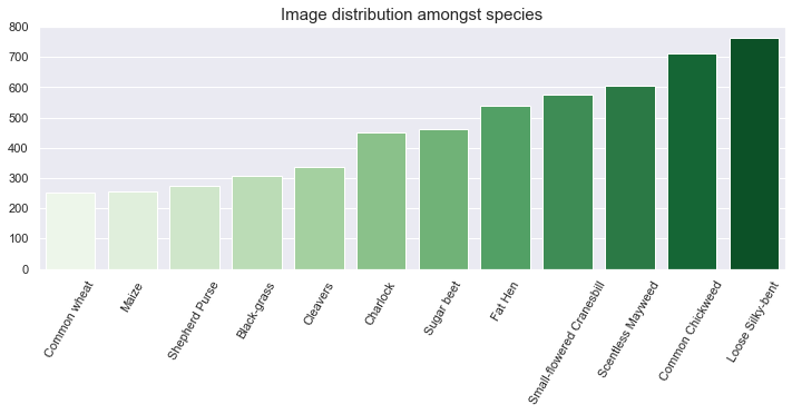
The above figure depicts an unbalanced dataset. Indeed, there is a three-time factor between the most common class (Loose Silky-bent) and the least common class (Common wheat).
The agricultural plants (wheat, maize, beet) are less present in the dataset compared to wild weeds.

fig, axes = plt.subplots(12, 5, figsize=(15, 45))
for n, folder in enumerate(listdir(ZIPEXTRACT)):
    # select random images from class
    image_names = np.random.choice(
        np.array(listdir(ZIPEXTRACT + folder + '/')), 5)
    for m, image_name in enumerate(image_names):
        image = imageio.imread(ZIPEXTRACT + folder + '/' + image_name)
        axes[n, m].imshow(image)
        axes[n, m].grid(False)
        axes[n, m].set_title(folder + '/' + image_name[0:-4])

Observations - Data content

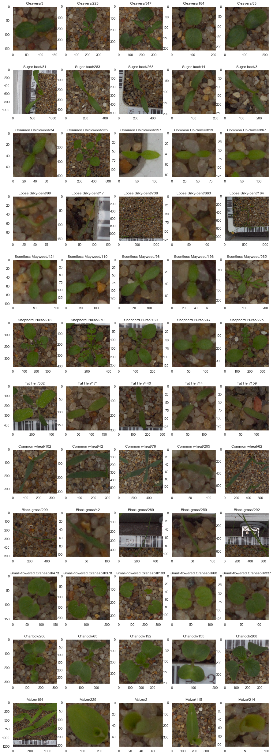
A few observations from each class are depicted in the above figure. The following observations can be made:

All images are top-down photographs.
The images have different sizes. This will have to be investigated.
If we assume that the soil gravels have the same size in all picture, it appears that the images are taken at various distances from the plants. This can create several issues with the model: a. The size of the gravels can be interpreted to classify a plant if certain species are consistently being photographed from the same distance. b. If the distance from the camera varies within a class, it can create confusion in the model as the definition of the plants will be different.
Some pictures are out of focus. This is an issue as shape detection becomes harder with blurry edges.
Several other components can be identified on the pictures. If these only appear with certain species, the model might learn to identify certain species based on the presence of unrelated components such as: a. Gravels b. Tags c. Rulers or dividers
The images have been taken at various step of the growth cycle of the plants. For instance, for the same species, some pictures show a single leaf while other shows more mature specimen with multiple large leaves.

Data Investigation

File Number vs Image Size

Prior to investigating the relationships between file number, image shape, and image resolution, we import the data into a pandas DataFrame to facilitate our analysis.

# instantiate main DataFrame
resolution_df = pd.DataFrame(
    columns=['file_name', 'species', 'width', 'height'])

# extract image information
for folder in listdir(ZIPEXTRACT):
    for file in listdir(ZIPEXTRACT + folder):
        image = imageio.imread(ZIPEXTRACT + folder + '/' + file)
        resolution_df = resolution_df.append(
            {
                'file_name': file,
                'species': folder,
                'width': float(image.shape[1]),
                'height': float(image.shape[0])
            },
            ignore_index=True)

# compute image ratio
resolution_df['ratio'] = resolution_df['width'] / resolution_df['height']

# isolate file number
resolution_df['file_num'] = resolution_df['file_name'].str.extract(
    r'(\d+)').astype(np.int16)

# print head to confirm extraction
resolution_df.head()

	file_name	species	width	height	ratio	file_num
0	348.png	Cleavers	450.0	450.0	1.0	348
1	176.png	Cleavers	295.0	295.0	1.0	176
2	88.png	Cleavers	299.0	299.0	1.0	88
3	162.png	Cleavers	194.0	194.0	1.0	162
4	189.png	Cleavers	438.0	438.0	1.0	189

The data has been imported into a dataframe. We have created two new features:

Image ratio - Ratio between image width and image height
File number - Number associated to the image

resolution_df.describe()

	width	height	ratio	file_num
count	5539.000000	5539.000000	5539.000000	5539.000000
mean	355.202022	354.783535	1.000231	267.794187
std	295.108600	292.700461	0.007453	183.276616
min	49.000000	49.000000	0.943368	1.000000
25%	152.000000	152.000000	1.000000	118.000000
50%	267.000000	267.000000	1.000000	236.000000
75%	469.000000	469.000000	1.000000	394.000000
max	3652.000000	3457.000000	1.332083	805.000000

We can now create several investigation to establish whether of not the file numbers have been assigned randomly.

fig, axes = plt.subplots(4, 3, figsize=(18, 15), sharex=True, sharey=True)

for idx, plant in enumerate(resolution_df['species'].unique()):
    row = idx % 4
    col = idx // 4

    axes[row, col].scatter(
        x=resolution_df.loc[resolution_df['species'] == plant, 'file_num'],
        y=resolution_df.loc[resolution_df['species'] == plant, 'width'],
        c=[sns.color_palette("hls", 12)[idx]],
        alpha=0.5)
    axes[row, col].set_title(plant, fontsize=15)

plt.tight_layout()

Observations

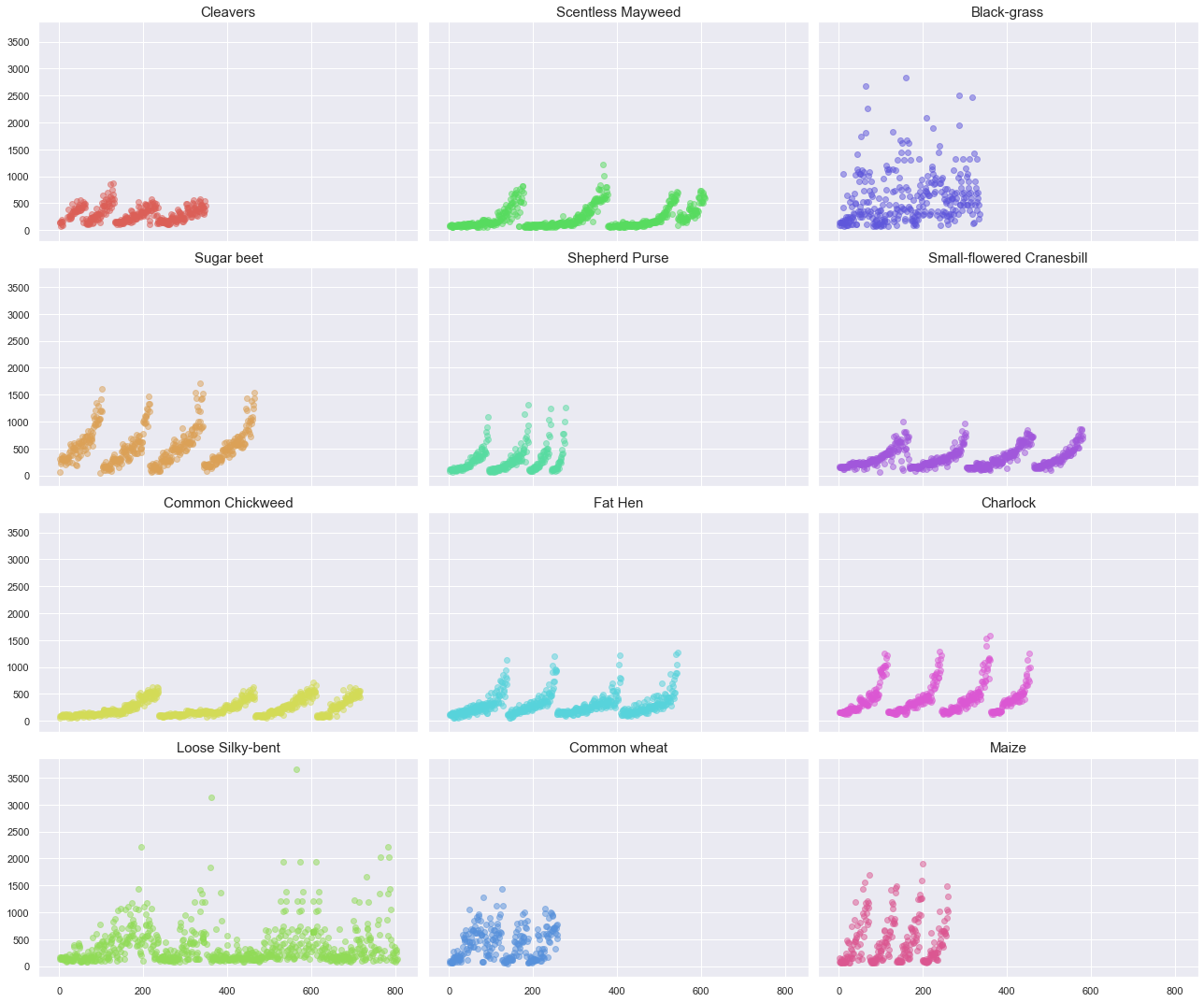
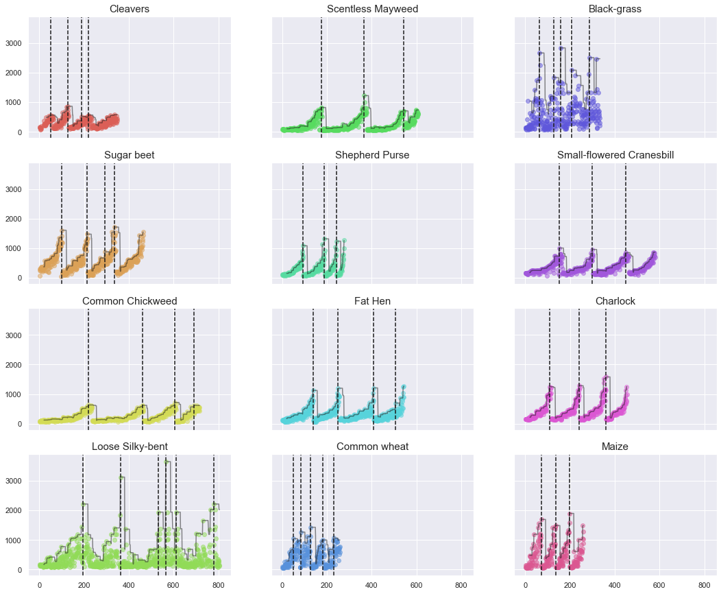
The first important observation is related to the number of files and the maximum resolution per plant. As shown in the above plot, the maximum resolution greatly varies between classes (~3000 pixel width for “Black-grass” vs. ~1000 pixel width for “Cleavers”).

A pattern appears when plotting the image width against the file number. As the file number increases, the width of the image increases up to a certain point, then the image size abruptly decreases. The pattern repeats approximately four times per species. Note that the pattern is not as well defined for the Back-grass and the Loose Silky bent species.

From this observation, we can make the following assumptions:

Four different plant specimens have been photographed at various stage of their growth cycles.
Four batches of specimens have been photographed simultaneously during their growth. Once the specimen are matured enough, they stopped being photographed.

We now need to create additional visualizations to validate our hypotheses.

There is one aspect of the data distribution to account for. Indeed, the trends are not perfect and some noise is clearly visible. In order to identify the file number corresponding to the beginning of a new resolution cycle, we are applying a rolling average.

# define a drop ratio between batches
max_ratio = 0.5

# store the file number corresponding to drop in resolution
cutoff_df = pd.DataFrame(columns=['species', 'drop'])

# prepare plot
fig, axes = plt.subplots(4, 3, figsize=(18, 15), sharex=True, sharey=True)

# iterate over each plant
for idx, plant in enumerate(resolution_df['species'].unique()):

    # sort per file num
    plant_df = resolution_df.loc[resolution_df['species'] ==
                                 plant].sort_values(by='file_num')

    # rolling max
    window = 20
    plant_df['roll_max_width'] = plant_df['width'].rolling(
        window, min_periods=window).max()

    # find drop
    drops = plant_df.loc[
        (plant_df['roll_max_width'] ==
         plant_df['roll_max_width'].shift(-window + 1)) &
        (plant_df['roll_max_width'] > plant_df['roll_max_width'].shift(1)) &
        (plant_df['roll_max_width'] > plant_df['roll_max_width'].max() *
         max_ratio), 'file_num']

    cutoff_df = cutoff_df.append({
        'species': plant,
        'drop': drops.to_list()
    },
                                 ignore_index=True)

    row = idx % 4
    col = idx // 4

    axes[row, col].plot(plant_df.loc[:, 'file_num'],
                        plant_df.loc[:, 'roll_max_width'],
                        c='k',
                        linestyle='-',
                        alpha=0.5)
    axes[row, col].set_title(plant)

    for drop_val in cutoff_df.loc[cutoff_df['species'] == plant, 'drop'].all():
        axes[row, col].axvline(drop_val, c='k', linestyle='--')

    axes[row, col].scatter(x=plant_df.loc[:, 'file_num'],
                           y=plant_df.loc[:, 'width'],
                           c=[sns.color_palette("hls", 12)[idx]],
                           alpha=0.5)
    axes[row, col].set_title(plant, fontsize=15)

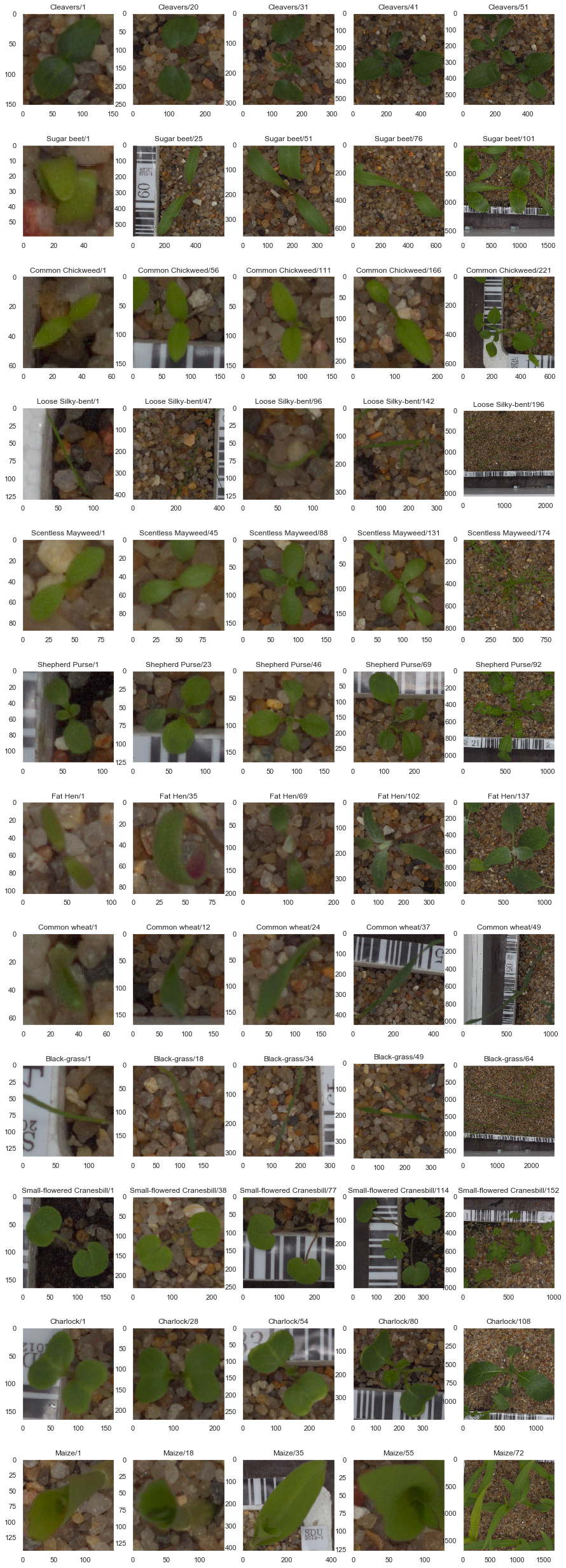
We can now plot various photographs per cycle and determine if there is any correlation (same seedling, same growth stage).

# create plot
fig, axes = plt.subplots(12, 5, figsize=(15, 45))

for idx, plant in enumerate(resolution_df['species'].unique()):

    # isolate first cycle cutoff
    cutoff_num = cutoff_df.loc[cutoff_df['species'] ==
                               plant, 'drop'].values[0][0]

    # isolate file numbers less that cutoff_num
    all_file_nums = resolution_df.loc[(resolution_df['species'] == plant) & (
        resolution_df['file_num'] <= cutoff_num)].sort_values(
            by='file_num')['file_num']

    # select images at 0%, 25%, 50%, 75%, and 100% of cycle
    selected_file_nums = all_file_nums.quantile([0., 0.25, 0.50, 0.75,
                                                 1.00]).astype(int).values

    # plot images
    for m, file_num in enumerate(selected_file_nums):
        # some images contain an underscore in the file name
        try:
            image = imageio.imread(ZIPEXTRACT + plant + '/' + str(file_num) +
                                   '.png')
        except:
            image = imageio.imread(ZIPEXTRACT + plant + '/' + str(file_num) +
                                   '-1.png')

        # plot image, hide grid, set title
        axes[idx, m].imshow(image)
        axes[idx, m].grid(False)
        axes[idx, m].set_title(plant + '/' + str(file_num))

Observations

For the above plots and displayed photographs, a clear relationship can be identified between file number and plant size (photo size). We can later leverage this information to extract a new feature corresponding to the seedling size.
We can hypothesize that the original photographs were taken at full resolution and that seedlings were manually cropped to create the individual images.

Image Shape and Resolution

Investigation

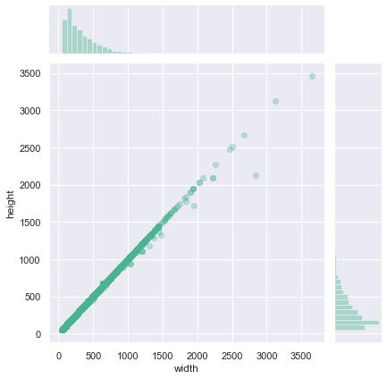
As previously established, the image sizes range from 49 pixels to 3652 pixels. This is an extreme difference that will impact the model. We are now going to dig deeper and investigate if the image size is correlated to the classes and if the set contains outliers.

sns.jointplot(x='width', y='height', data=resolution_df, color="#4CB391", alpha=0.3);

print(
    "Pearson correlation between image height and image width: {:.5f}".format(
        resolution_df[['width', 'height']].corr().iloc[0, 1]))

Pearson correlation between image height and image width: 0.99922

print("{:.2f}% of the images are square (ratio=1.)".format((resolution_df['ratio']==1).mean()*100))

98.77% of the images are square (ratio=1.)

Observations

From the above distribution plot, it appear that most of the images present a 1:1 shape ratio. We can now filter the square images and search for additional information using the non-square images.

fig, ax = plt.subplots(figsize=(18, 6))
sns.boxplot(x="species", y="width", data=resolution_df, ax=ax)
plt.xticks(rotation=45)
ax.set_title('Distribution of image width between species', fontsize=15)

Text(0.5, 1.0, 'Distribution of image width between species')

Observations

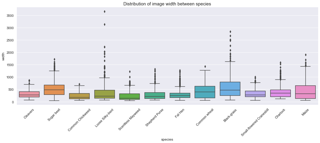
The above boxplot shows the followings:

Each class contains outliers with large width.
The width distribution is not consistent between classes.
The minimum width seems to be roughly identical between classes (~60 pixels) except for the “Charlock” class.

print('Minimum image height and width across species:')
print(resolution_df.groupby(['species'])[['width','height']].min())

Minimum image height and width across species:
                           width  height
species                                 
Black-grass                 73.0    73.0
Charlock                   121.0   121.0
Cleavers                    66.0    66.0
Common Chickweed            54.0    54.0
Common wheat                51.0    51.0
Fat Hen                     55.0    55.0
Loose Silky-bent            71.0    71.0
Maize                       54.0    54.0
Scentless Mayweed           49.0    49.0
Shepherd Purse              63.0    63.0
Small-flowered Cranesbill   62.0    62.0
Sugar beet                  49.0    49.0

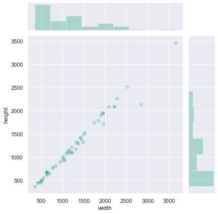
We previously saw that most of the images are square. We can focus on the rectangular image to see if there is a pattern in their distribution (species, size).

filtered_df = resolution_df[resolution_df['ratio'] != 1.00]
sns.jointplot(x='width', y='height', data=filtered_df, color="#4CB391", alpha=0.3);

print(
    "Pearson correlation between image height and image width for rectangular images: {:.5f}".format(
        filtered_df[['width', 'height']].corr().iloc[0, 1]))

Pearson correlation between image height and image width for rectangular images: 0.99013

Observations

The height/width of rectangular images are distributed is a manner similar as the rest of the data.

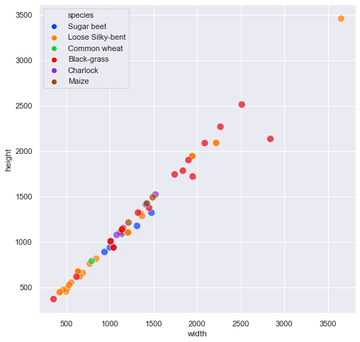
fig, ax = plt.subplots(figsize=(8, 8))
sns.scatterplot(x='width',
                y='height',
                data=filtered_df,
                color="#4CB391",
                alpha=0.7,
                hue='species',
                s=100,
                palette=sns.color_palette("bright", 6));

Observations

From the above plots, we can draw the following observations:

Most of the rectangular images from the “Loose Silky-bent” are small images <700pixels)
Eventhough these images are not perfectly square, they are fairly square (correlation of 0.99).

fig, ax = plt.subplots(2, 1, figsize=(16, 12))
for single in resolution_df.species.unique():
    sns.kdeplot(resolution_df[resolution_df['species'] == single].width,
                ax=ax[0],
                label=single)
ax[0].legend()
ax[0].set_title("KDE-Plot of image width given species", fontsize=15)
ax[0].set_xlabel("Image width")
ax[0].set_ylabel("Density")
sns.distplot(resolution_df.width, ax=ax[1], color="#4CB391", hist_kws={'alpha':0.8}, kde_kws={'color':'k'})
ax[1].set_xlabel("Image width")
ax[1].set_ylabel("Density")
ax[1].set_title("Overall image width distribution", fontsize=15)
plt.tight_layout()

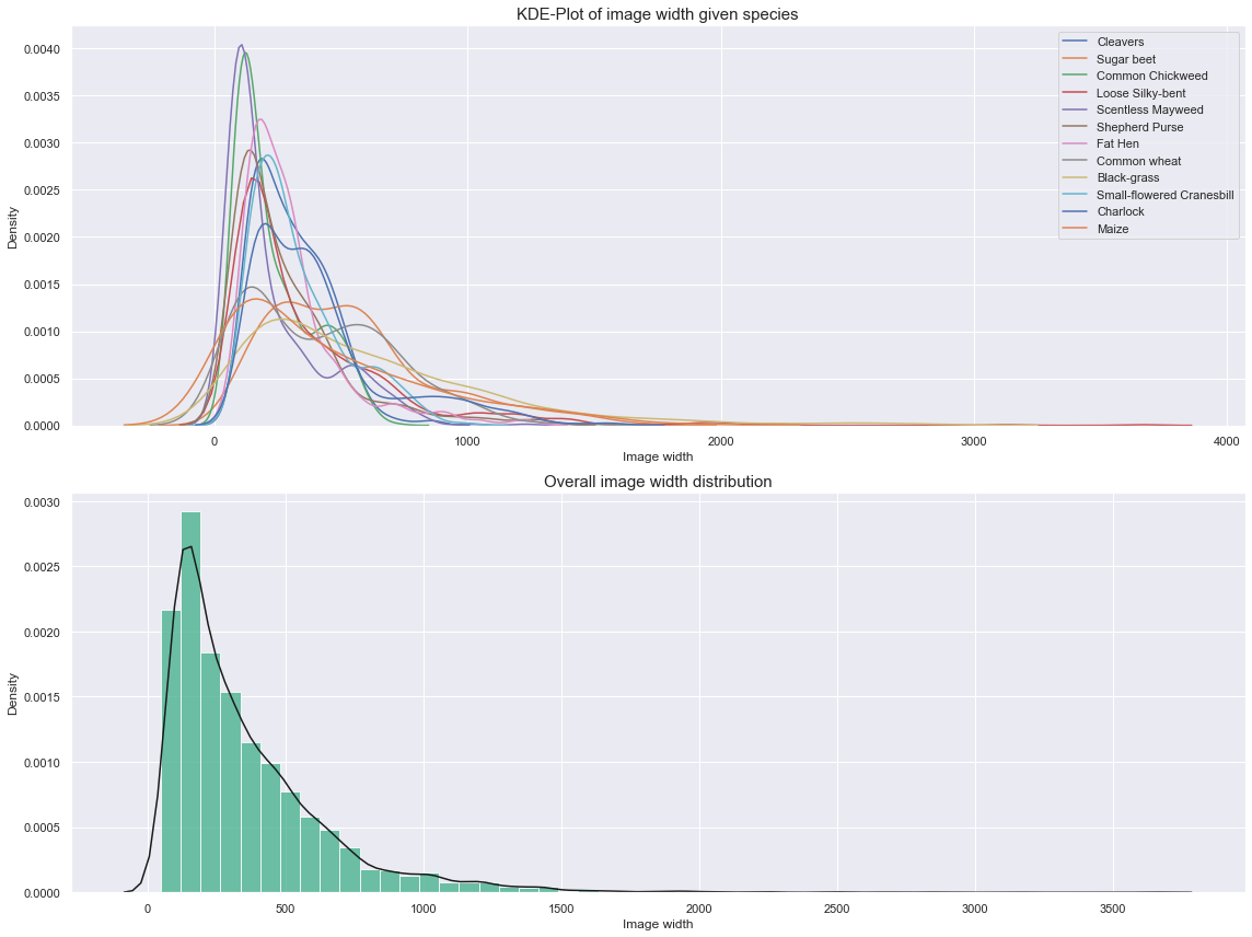
The above plots show distribution that are typical for log distribution. We can apply a log transformation to normalize them.

fig, ax = plt.subplots(2, 1, figsize=(16, 12))
for single in resolution_df.species.unique():
    sns.kdeplot(np.log(
        resolution_df[resolution_df['species'] == single].width),
                ax=ax[0],
                label=single)
ax[0].legend()
ax[0].set_title("KDE-Plot of image width given species", fontsize=15)
ax[0].set_xlabel("Image width")
ax[0].set_ylabel("Density")
sns.distplot(np.log(resolution_df.width), ax=ax[1], color="#4CB391", hist_kws={'alpha':0.8}, kde_kws={'color':'k'})
ax[1].set_xlabel("Image width")
ax[1].set_ylabel("Density")
ax[1].set_title("Overall image width distribution", fontsize=15)
plt.tight_layout()

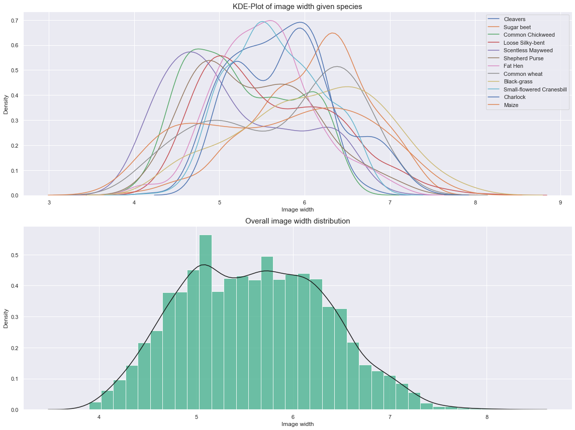
Observations

Three groups can be identified from the above plots.
These groups are highly tied to a subset of species. This could be a valuable add-on to our model.

Feature Engineering

During our investigation, we have reached the following conclusions:

The image size can be a good indicator of the plant species.
For each species, we have identified image cycles through the file names. We have extracted approximate cut-off for each cycle and each species.
Each image contains a certain number of external components that can contaminate the model.

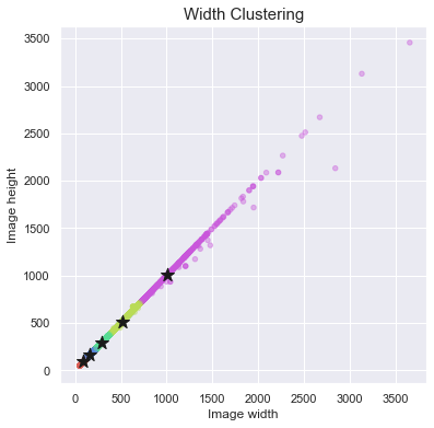
One of the first focus of our feature engineering is going to try to estimate the growth state. To do so, we will cluster the width of the images.

Note: since we have established that most of the images are square, we are only going to use the width as our main feature from now on.

# normalize and scale the data
scaler = StandardScaler()

X = np.log(resolution_df['width'].values).reshape(-1,1)
X = scaler.fit_transform(X)

K = range(3, 20)
inertias = []

for k in tqdm_notebook(K):
    km = KMeans(n_clusters=k)
    km.fit(X)
    
    # compute inertias
    inertias.append(km.inertia_) 

HBox(children=(IntProgress(value=0, max=17), HTML(value='')))

plt.figure(figsize=(12, 6))
plt.plot(K, inertias, 'X-', markersize=10, color="#4CB391")
plt.xlabel('Values of K')
plt.ylabel('Inertia')
plt.title('The Elbow Method using Inertia', fontsize=15)
plt.show()

Observations

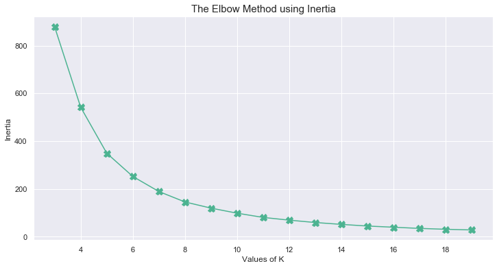
Using the elbow method on the inertia, we can consider 5 to be an appropriate number of clusters for our growth cycle.

# re-train KMeans using optimal number of clusters
km = KMeans(n_clusters=5, random_state=10)

# assign cluster to records
resolution_df['growth_lvl'] = km.fit_predict(X)

fig, ax = plt.subplots(1, 1, figsize=(6, 6))

colors = resolution_df['growth_lvl'].apply(
    lambda x: sns.color_palette("hls", 5)[x]).values

ax.scatter(resolution_df['width'].values,
           resolution_df['height'].values,
           s=20,
           c=colors,
           alpha=0.4)
ax.set_xlabel("Image width")
ax.set_ylabel("Image height")
ax.set_title("Width Clustering", fontsize=15)

for cluster_center in np.exp(scaler.inverse_transform((km.cluster_centers_))):
    ax.scatter(x=cluster_center, y=cluster_center, marker='*', c='k', s=160)

fig, axes = plt.subplots(4, 3, figsize=(18, 15), sharex=True, sharey=True)

for idx, plant in enumerate(resolution_df['species'].unique()):
    row = idx % 4
    col = idx // 4

    colors = [
        sns.color_palette("hls", 5)[x] for x in
        resolution_df.loc[resolution_df['species'] == plant, 'growth_lvl']
    ]

    axes[row, col].scatter(
        x=resolution_df.loc[resolution_df['species'] == plant, 'file_num'],
        y=resolution_df.loc[resolution_df['species'] == plant, 'width'],
        c=colors,
        alpha=0.5)

    axes[row, col].set_title(plant, fontsize=15)

    if row == 0 and col == 0:
        legend_elements = [
            Line2D([0], [0],
                   marker='o',
                   linewidth=0,
                   markeredgecolor=sns.color_palette('hls', 5)[x],
                   label='Cluster ' + str(x),
                   markerfacecolor=sns.color_palette('hls', 5)[x],
                   markersize=10) for idx, x in enumerate(range(5))
        ]
        axes[row, col].legend(handles=legend_elements, loc='upper right')

plt.tight_layout()

for idx, k in enumerate(np.exp(scaler.inverse_transform((km.cluster_centers_))).reshape(1,-1)[0]):
    print('Cluster {}: width = {:.1f}'.format(idx, k))

Cluster 0: width = 93.7
Cluster 1: width = 517.8
Cluster 2: width = 294.4
Cluster 3: width = 166.0
Cluster 4: width = 1008.7

CLUSTER_ORDER = km.cluster_centers_.reshape(1,-1).argsort().tolist()[0]
CLUSTER_ORDER

[0, 3, 2, 1, 4]

Observations

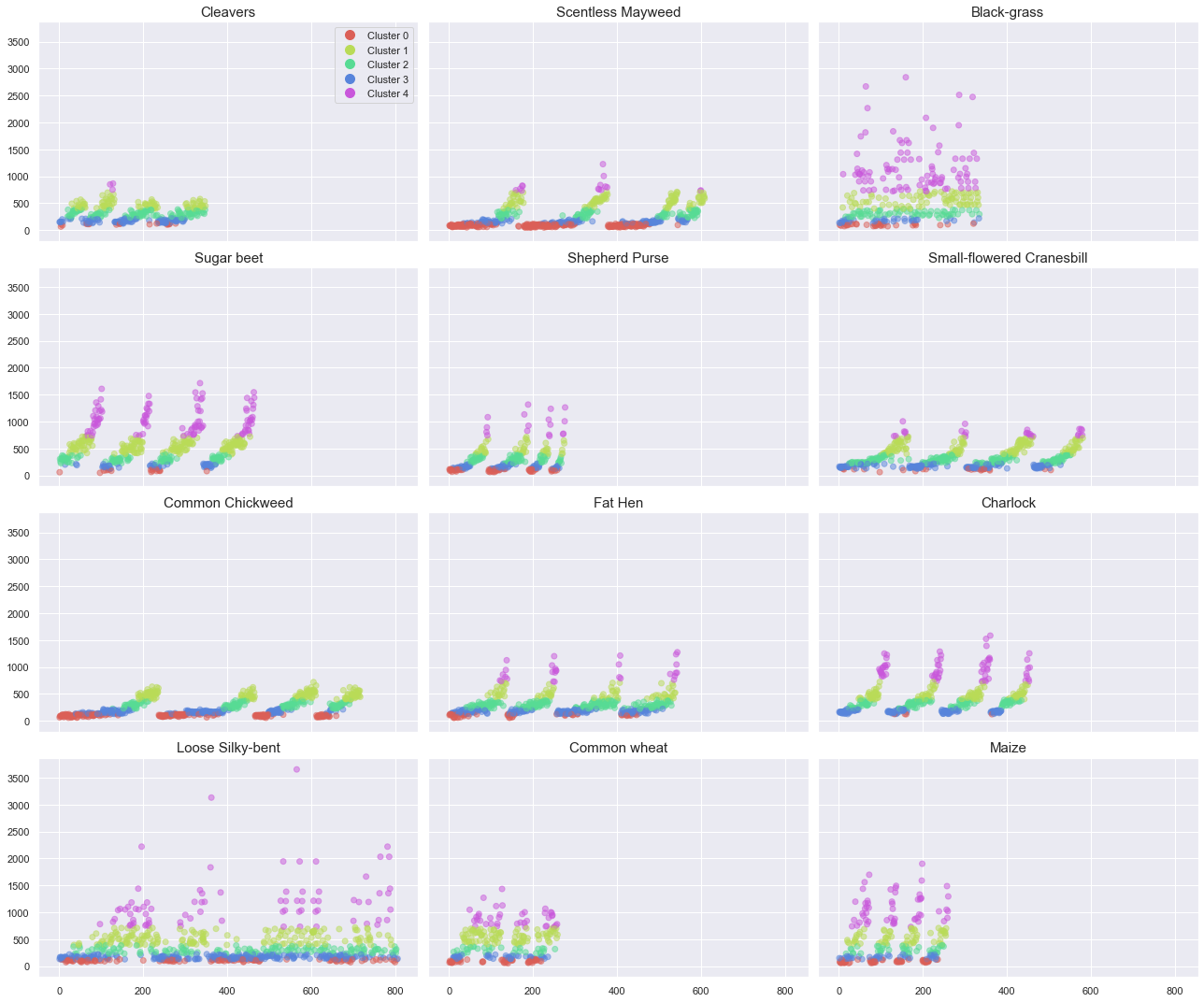
The above plots show the results of our clustering. We can make the following observations:

most plant present photographs in the 5 clusters.
for each plant, the repetition of growth cycle through each period (file numbers) are identical.

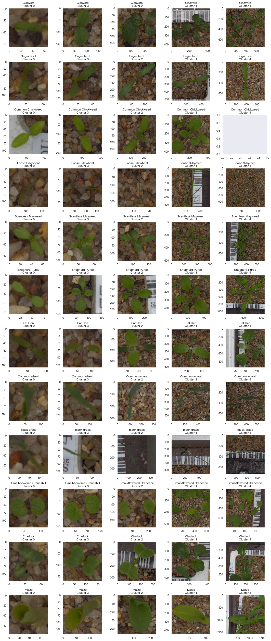
We can now plot individual of each cycle and validate our assumptions.

# create plot
fig, axes = plt.subplots(12, 5, figsize=(15, 35))

# iterate over species
for idx, plant in enumerate(resolution_df['species'].unique()):

    # iterate over clusters
    for n, cycle in enumerate(CLUSTER_ORDER):

        # select subset
        filtered_df = resolution_df.loc[(resolution_df['species'] == plant) &
                                        (resolution_df['growth_lvl'] == cycle)]

        # select random image
        if filtered_df.shape[0] > 0:
            file_name = filtered_df.sample(1)['file_name'].values[0]

            image = imageio.imread(ZIPEXTRACT + plant + '/' + file_name)

            # plot image, hide grid, set title
            axes[idx, n].imshow(image)
        axes[idx, n].grid(False)
        axes[idx, n].set_title(plant + '\n' + 'Cluster ' + str(cycle))
        
plt.tight_layout()

We also would like to obtain the count of photographs per species and per cluster.

CLUSTER_ORDER_str = [str(x) for x in CLUSTER_ORDER]

# aggregate by species and growth_lvl
agg_df = resolution_df.groupby(['growth_lvl', 'species']).size().unstack().fillna(0)
agg_df.index = agg_df.index.astype(str)

# compute percentable per species
agg_df = agg_df / resolution_df['species'].value_counts()

agg_df = agg_df.iloc[CLUSTER_ORDER, :]

plt.figure(figsize=(16, 6))
sns.heatmap(agg_df.reindex(CLUSTER_ORDER_str),
            annot=True,
            fmt=".0%",
            xticklabels='auto',
            cmap='BuGn',
            annot_kws={"size": 15},
            cbar=False)
plt.ylim(0, 5)
plt.yticks(rotation=90)
plt.xticks(rotation=60)
plt.title("Cluster distribution per species", fontsize=15);

Observations

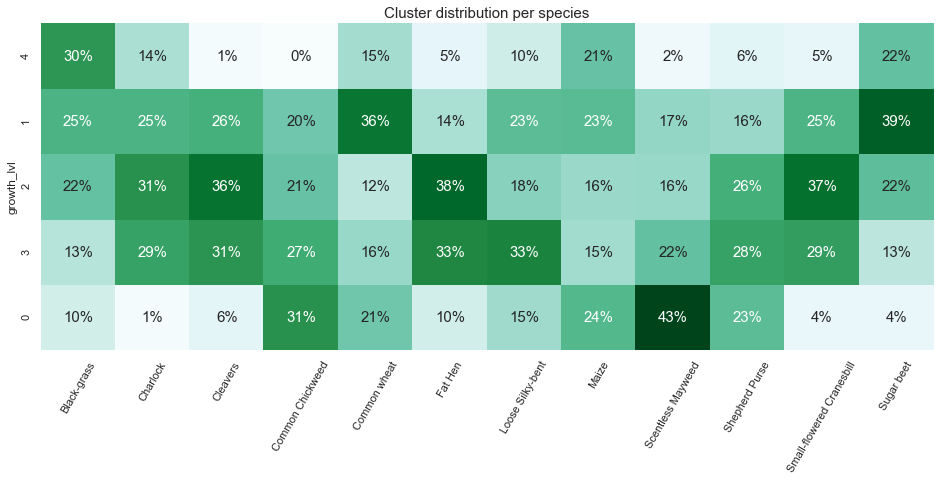
The new growth cycle cluster appears to be a good feature for certain species. For instance 43% of the “Scentless Mayweed” can be found in cluster 0. In addition, some cluster barely contain any individual for certain species.
This finding can be considered as data leakage and our model may be tempted to predict a class based on the size of the image. Something will have to be done to prevent such a flaw.
Finally, we observed early on, a class imbalance. The imbalance combined with the leakage can become really problematic and will both need to be addressed.

Convolutional Neural Network

In this section, we will train a CNN to predict the species feature. The approach is divided between the following steps:

Encode the target feature
Download the data
Split the data between a training and test set
Perform data augmentation
Determine the cost function to be optimized

Data Loader, Validation and Data Augmentation

In order for our model to generalize well on unseen data, a good practice consists of using image transformation to create new unseen examples.
We need to ensure that our model does not over fit the training data. To do so, we are using a training set and a test set both taken from the original dataset.

Keras contains useful tools to help process image files and feed them in batches to the model. We will be using a generator for both the train and test phases.

First, we must create a new feature to our dataset which contains the full path to each image.
Then, we can create two generators, the training generator will contains several data augmentation transformation (horizontal and vertical flips, zoom).
Both the train and test generator will normalize the pixel values.
Finally, the images will be sent to the model using batches of 32 RGB images reshaped at 70x70.

# create full path to data
resolution_df['full_path'] = '../Data/' + resolution_df[
    'species'] + '/' + resolution_df['file_name']
resolution_df.head()

	file_name	species	width	height	ratio	file_num	growth_lvl	full_path
0	348.png	Cleavers	450.0	450.0	1.0	348	1	../Data/Cleavers/348.png
1	176.png	Cleavers	295.0	295.0	1.0	176	2	../Data/Cleavers/176.png
2	88.png	Cleavers	299.0	299.0	1.0	88	2	../Data/Cleavers/88.png
3	162.png	Cleavers	194.0	194.0	1.0	162	3	../Data/Cleavers/162.png
4	189.png	Cleavers	438.0	438.0	1.0	189	1	../Data/Cleavers/189.png

# image size
scale = 224

# batch size
batch_size = 32

# random seed
seed = 10

At this point of the analysis, the images have not been loaded into a numpy array. Using the data stored in the pandas DataFrame, we load the images into a single array of size (N, scale, scale).

# load images into a numpy array
full_set = []
for i in tqdm_notebook(resolution_df['full_path']):
    full_set.append(cv2.resize(cv2.imread(i)[:,:,::-1],(scale,scale)))
full_set = np.asarray(full_set)

print("{} images in full set.".format(full_set.shape[0]))

HBox(children=(IntProgress(value=0, max=5539), HTML(value='')))

5539 images in full set.

Now that the images have been loaded and resized, we have to work on the target labels. The current feature used to encode the species contains various strings. We need to convert the list of labels into a one-hot encoded array of size (N, n) where n is the number of species in the dataset.

# encode target
# create encoder and fit on training set
labels = LabelEncoder()
labels.fit(resolution_df['species'])

# display target classes
print('Classes'+str(labels.classes_))

# encode labels
encodedlabels = labels.transform(resolution_df['species'])
clearalllabels = np_utils.to_categorical(encodedlabels)

# store number of classes for future use
n_classes = clearalllabels.shape[1]

Classes['Black-grass' 'Charlock' 'Cleavers' 'Common Chickweed' 'Common wheat'
 'Fat Hen' 'Loose Silky-bent' 'Maize' 'Scentless Mayweed' 'Shepherd Purse'
 'Small-flowered Cranesbill' 'Sugar beet']

Before we can feed our data into a model, an essential step consists of scaling the pixel values down to range from 0 to 1. This will stabilize the training of the model. Since RGB encoding ranges from 0 to 255, we will divide the pixel values by 255.

# scale data
full_set = full_set / 255.

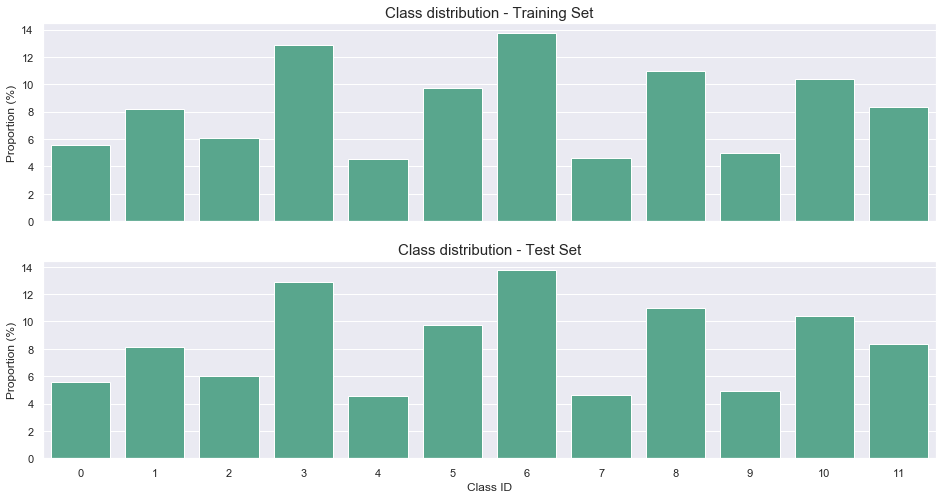
Finally, we need to establish our validation strategy. We divide the entire set of images into a training set (90%) and a test set (10%). Since the classes are unbalanced, we are forcing the train-test-split to be as consistent as possible by stratifying the selection process.

# isolate train and test indexes
X_train, X_test, y_train, y_test = train_test_split(full_set,
                                                    clearalllabels,
                                                    test_size=0.1,
                                                    random_state=seed,
                                                    stratify=resolution_df['species'])

# plot proportions
train_split = pd.Series(y_train.argmax(axis=1)).value_counts()/y_train.shape[0]*100
test_split = pd.Series(y_test.argmax(axis=1)).value_counts()/y_test.shape[0]*100

fig, axes = plt.subplots(2,1,figsize=(16, 8), sharex=True)
sns.barplot(train_split.index, train_split, color='#4CB391', ax=axes[0])
sns.barplot(test_split.index, train_split, color='#4CB391', ax=axes[1])
axes[0].set_title("Class distribution - Training Set", fontsize=15)
axes[1].set_title("Class distribution - Test Set", fontsize=15)
axes[0].set_ylabel('Proportion (%)')
axes[1].set_ylabel('Proportion (%)')
axes[1].set_xlabel("Class ID");

Finally, we will use data augmentation to help the model generalize on unseen data. The following actions can be taken:

Rotation from -180 to 180 deg
Width and height shifts of 10%
Shear range of 10%
Zoom range of 10%
Horizontal and vertical flips

# data augmentation
generator = ImageDataGenerator(rotation_range=180,
                               width_shift_range=0.1,
                               height_shift_range=0.1,
                               brightness_range=None,
                               shear_range=0.0,
                               zoom_range=0.1,
                               channel_shift_range=0.0,
                               fill_mode='nearest',
                               horizontal_flip=True,
                               vertical_flip=True,
                               dtype='float32')

Build Model

It is now time to build our model. We will use a Convolutional Neural Network (CNN). The three CNN blocks are defined as follows:

Conv2D + relu
BatchNorm
Conv2D + relu
Maxpooling
BatchNorm
Dropout

The CNN is followed by two dense layers equipped with BatchNorm and Dropout.

np.random.seed(seed)

model = Sequential()

model.add(Conv2D(filters=32, kernel_size=(5, 5), input_shape=(scale, scale, 3), activation='relu'))
model.add(BatchNormalization(axis=3))
model.add(Conv2D(filters=64, kernel_size=(5, 5), activation='relu'))
model.add(MaxPooling2D((2, 2)))
model.add(BatchNormalization(axis=3))
model.add(Dropout(0.1))

model.add(Conv2D(filters=64, kernel_size=(5, 5), activation='relu'))
model.add(BatchNormalization(axis=3))
model.add(Conv2D(filters=64, kernel_size=(5, 5), activation='relu'))
model.add(MaxPooling2D((2, 2)))
model.add(BatchNormalization(axis=3))
model.add(Dropout(0.1))

model.add(Conv2D(filters=128, kernel_size=(5, 5), activation='relu'))
model.add(BatchNormalization(axis=3))
model.add(Conv2D(filters=128, kernel_size=(5, 5), activation='relu'))
model.add(MaxPooling2D((2, 2)))
model.add(BatchNormalization(axis=3))
model.add(Dropout(0.1))

model.add(Conv2D(filters=256, kernel_size=(5, 5), activation='relu'))
model.add(BatchNormalization(axis=3))
model.add(Conv2D(filters=256, kernel_size=(5, 5), activation='relu'))
model.add(MaxPooling2D((2, 2)))
model.add(BatchNormalization(axis=3))
model.add(Dropout(0.1))

model.add(Flatten())

model.add(Dense(256, activation='relu'))
model.add(BatchNormalization())
model.add(Dropout(0.5))

model.add(Dense(256, activation='relu'))
model.add(BatchNormalization())
model.add(Dropout(0.5))

model.add(Dense(n_classes, activation='softmax'))

Metric Definition and Optimizer

Before we can train our model, we have to define the followings:

Optimizing metrics: in our case, we will be optimizing the cross-entropy. This is typical for a multi-class problem.
Optimizer technique: an Adam optimizer is used.
Optimization strategy: that is how to adjust the learning rate, when to stop the training.

# optimizer
optimizer = optimizers.Adam(lr=1e-3, beta_1=0.9, beta_2=0.999)

# define loss function
model.compile(optimizer=optimizer,
              loss=losses.categorical_crossentropy,
              metrics=['acc'])

# define optimization schedule with callbacks
lrate = ReduceLROnPlateau(monitor='val_acc',
                          factor=0.4,
                          patience=3,
                          verbose=1,
                          min_lr=0.0001)

filepath = "./Model_0/weights.best_{epoch:02d}-{val_acc:.2f}.hdf5"
checkpoints = ModelCheckpoint(filepath,
                              monitor='val_acc',
                              verbose=1,
                              save_best_only=False,
                              period=1)

callbacks_list = [lrate, checkpoints, TQDMNotebookCallback(leave_inner=False, leave_outer=True)]

model.summary()

Model: "sequential_1"
_________________________________________________________________
Layer (type)                 Output Shape              Param #   
=================================================================
conv2d_1 (Conv2D)            (None, 220, 220, 32)      2432      
_________________________________________________________________
batch_normalization_1 (Batch (None, 220, 220, 32)      128       
_________________________________________________________________
conv2d_2 (Conv2D)            (None, 216, 216, 64)      51264     
_________________________________________________________________
max_pooling2d_1 (MaxPooling2 (None, 108, 108, 64)      0         
_________________________________________________________________
batch_normalization_2 (Batch (None, 108, 108, 64)      256       
_________________________________________________________________
dropout_1 (Dropout)          (None, 108, 108, 64)      0         
_________________________________________________________________
conv2d_3 (Conv2D)            (None, 104, 104, 64)      102464    
_________________________________________________________________
batch_normalization_3 (Batch (None, 104, 104, 64)      256       
_________________________________________________________________
conv2d_4 (Conv2D)            (None, 100, 100, 64)      102464    
_________________________________________________________________
max_pooling2d_2 (MaxPooling2 (None, 50, 50, 64)        0         
_________________________________________________________________
batch_normalization_4 (Batch (None, 50, 50, 64)        256       
_________________________________________________________________
dropout_2 (Dropout)          (None, 50, 50, 64)        0         
_________________________________________________________________
conv2d_5 (Conv2D)            (None, 46, 46, 128)       204928    
_________________________________________________________________
batch_normalization_5 (Batch (None, 46, 46, 128)       512       
_________________________________________________________________
conv2d_6 (Conv2D)            (None, 42, 42, 128)       409728    
_________________________________________________________________
max_pooling2d_3 (MaxPooling2 (None, 21, 21, 128)       0         
_________________________________________________________________
batch_normalization_6 (Batch (None, 21, 21, 128)       512       
_________________________________________________________________
dropout_3 (Dropout)          (None, 21, 21, 128)       0         
_________________________________________________________________
conv2d_7 (Conv2D)            (None, 17, 17, 256)       819456    
_________________________________________________________________
batch_normalization_7 (Batch (None, 17, 17, 256)       1024      
_________________________________________________________________
conv2d_8 (Conv2D)            (None, 13, 13, 256)       1638656   
_________________________________________________________________
max_pooling2d_4 (MaxPooling2 (None, 6, 6, 256)         0         
_________________________________________________________________
batch_normalization_8 (Batch (None, 6, 6, 256)         1024      
_________________________________________________________________
dropout_4 (Dropout)          (None, 6, 6, 256)         0         
_________________________________________________________________
flatten_1 (Flatten)          (None, 9216)              0         
_________________________________________________________________
dense_1 (Dense)              (None, 256)               2359552   
_________________________________________________________________
batch_normalization_9 (Batch (None, 256)               1024      
_________________________________________________________________
dropout_5 (Dropout)          (None, 256)               0         
_________________________________________________________________
dense_2 (Dense)              (None, 256)               65792     
_________________________________________________________________
batch_normalization_10 (Batc (None, 256)               1024      
_________________________________________________________________
dropout_6 (Dropout)          (None, 256)               0         
_________________________________________________________________
dense_3 (Dense)              (None, 12)                3084      
=================================================================
Total params: 5,765,836
Trainable params: 5,762,828
Non-trainable params: 3,008
_________________________________________________________________

# Fit the model
history = model.fit_generator(generator.flow(X_train, y_train, batch_size=batch_size),
                    epochs=50,
                    steps_per_epoch=np.ceil(X_train.shape[0] / batch_size),
                    validation_data=(X_test, y_test),
                    callbacks=callbacks_list,
                    verbose=2)

Epoch 1/50 - 2586s - loss: 2.1630 - acc: 0.3713 - val_loss: 9.3464 - val_acc: 0.2022  
Epoch 2/50 - 2562s - loss: 1.4018 - acc: 0.5561 - val_loss: 1.7693 - val_acc: 0.5235  
Epoch 3/50 - 2554s - loss: 1.1133 - acc: 0.6468 - val_loss: 1.6343 - val_acc: 0.5505  
.  
.  
.  
Epoch 49/50 - 2746s - loss: 0.2220 - acc: 0.9234 - val_loss: 0.3810 - val_acc: 0.8736  
Epoch 50/50 - 2747s - loss: 0.2100 - acc: 0.9202 - val_loss: 0.2375 - val_acc: 0.9152  

lr = pd.read_csv('lr_0.csv', index_col=0)
history = pd.read_csv('history_0.csv', index_col=0)

fig, axes = plt.subplots(2, 2, figsize=(16, 12))
axes[0,0].plot(history['loss'], label='training', c='dodgerblue')
axes[0,0].plot(history['val_loss'], label='validation', c='crimson')
axes[0,0].legend()
axes[0,0].set_title("Loss function", fontsize=15)
axes[0,0].set_xlabel("epochs")
axes[0,0].set_ylabel("loss")

axes[0,1].plot(history['acc'], label='training', c='dodgerblue')
axes[0,1].plot(history['val_acc'], label='validation', c='crimson')
axes[0,1].legend()
axes[0,1].set_title("Accuracy", fontsize=15)
axes[0,1].set_xlabel("epochs")
axes[0,1].set_ylabel("accuracy")

axes[1,0].plot(lr['lr'], c='dodgerblue')
axes[1,0].set_title("Learning Rate", fontsize=15)
axes[1,0].set_xlabel("epochs")
axes[1,0].set_ylabel("learning rate")
axes[1,0].set_ylim(0,0.0011)

axes[-1,-1].axis('off');

Results

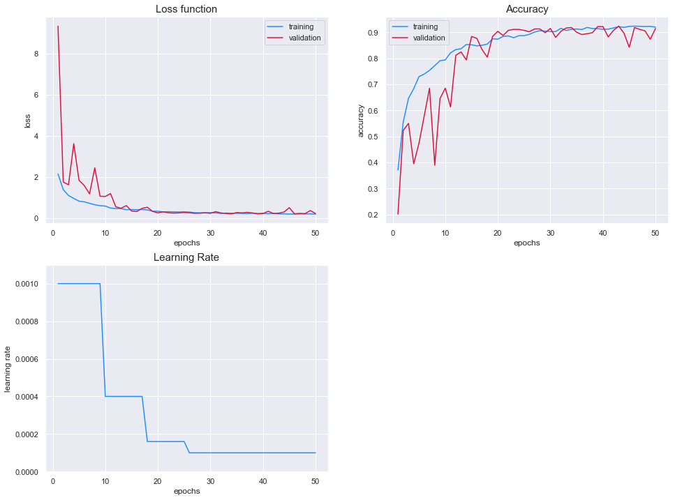
The value of the loss functions is almost identical between the two sets. We can see that the model has reached a stable configuration as the loss function of the training set and test set both plateau after 15 epochs.

In addition, the accuracy of both models reach around 90%.

In conclusion, the training of the model is considered to be successful. Overfitting has been prevented by using data augmentation techniques and the model performs well on both sets.

The next step is to investigate the performances of the model by looking at predictions.

Predictions and Results

print("Maximum accuray on validation step:")
print(" Epoch: {}".format(np.argmax(history['val_acc'])))
print("        {:.2f}%".format(history['val_acc'].values.max()*100))

Maximum accuray on validation step:
 Epoch: 43
        92.42%

# load best model
model.load_weights("./Model_0/weights.best_43-0.92.hdf5")

Make predictions on both the train and test sets.

y_train_pred = model.predict(X_train, verbose=1).argmax(axis=1)
y_test_pred = model.predict(X_test, verbose=1).argmax(axis=1)

print('Training Data')
ax = TAD_tools_v01.plot_confusion_matrix(y_train.argmax(axis=1),
                                    y_train_pred,
                                    labels.classes_,
                                    normalize=True,
                                    title=None,
                                    cmap=plt.cm.Oranges,
                                    figsize=(12,12))

ax.set_ylim(11.5,-0.5);

Training Data

print('Test Data')
ax = TAD_tools_v01.plot_confusion_matrix(y_test.argmax(axis=1),
                                    y_test_pred,
                                    labels.classes_,
                                    normalize=True,
                                    title=None,
                                    cmap=plt.cm.Greens,
                                    figsize=(12,12))

ax.set_ylim(11.5,-0.5);

Test Data

print("Accurancy:")
print("   Train: {:.2f}%".format(metrics.accuracy_score(y_train.argmax(axis=1), y_train_pred)*100))
print("   Test:  {:.2f}%".format(metrics.accuracy_score(y_test.argmax(axis=1), y_test_pred)*100))

print("\nF1-score")
print("   Train: {:.3f}%".format(metrics.f1_score(y_train.argmax(axis=1), y_train_pred, average='weighted')*100))
print("   Test:  {:.3f}%".format(metrics.f1_score(y_test.argmax(axis=1), y_test_pred, average='weighted')*100))

print("\nClassification Report")
print(metrics.classification_report(y_train.argmax(axis=1), y_train_pred))
print(metrics.classification_report(y_test.argmax(axis=1), y_test_pred))

Accurancy:
   Train: 93.68%
   Test:  92.78%

F1-score
   Train: 93.670%
   Test:  92.916%

Classification Report
              precision    recall  f1-score   support

           0       0.70      0.66      0.68       278
           1       0.97      0.98      0.98       407
           2       0.89      0.96      0.92       301
           3       0.99      0.94      0.97       642
           4       0.81      0.99      0.89       228
           5       0.99      0.98      0.98       484
           6       0.91      0.86      0.89       686
           7       0.99      0.97      0.98       231
           8       0.91      0.98      0.95       546
           9       0.98      0.91      0.95       247
          10       0.99      0.98      0.99       518
          11       0.99      0.97      0.98       417

    accuracy                           0.94      4985
   macro avg       0.93      0.93      0.93      4985
weighted avg       0.94      0.94      0.94      4985

              precision    recall  f1-score   support

           0       0.61      0.74      0.67        31
           1       0.93      0.93      0.93        45
           2       0.82      0.97      0.89        34
           3       0.99      0.94      0.96        71
           4       0.89      1.00      0.94        25
           5       1.00      0.98      0.99        54
           6       0.92      0.80      0.86        76
           7       1.00      1.00      1.00        26
           8       0.94      0.95      0.94        61
           9       1.00      0.89      0.94        27
          10       0.98      0.98      0.98        58
          11       0.98      0.98      0.98        46

    accuracy                           0.93       554
   macro avg       0.92      0.93      0.92       554
weighted avg       0.93      0.93      0.93       554

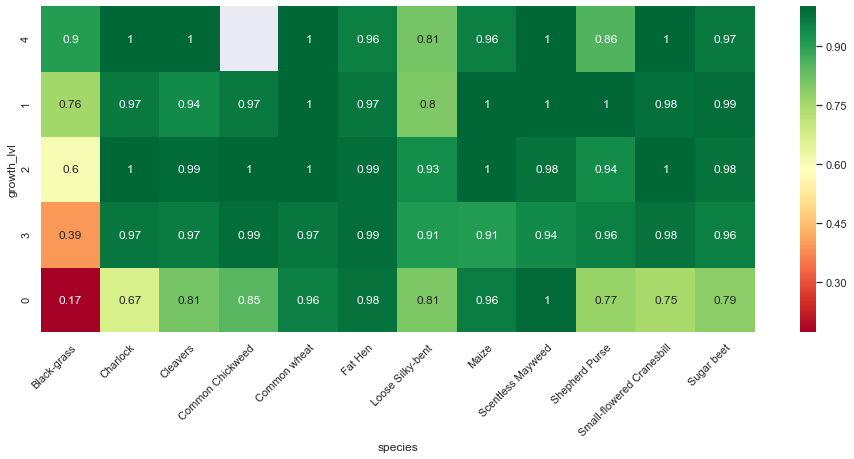
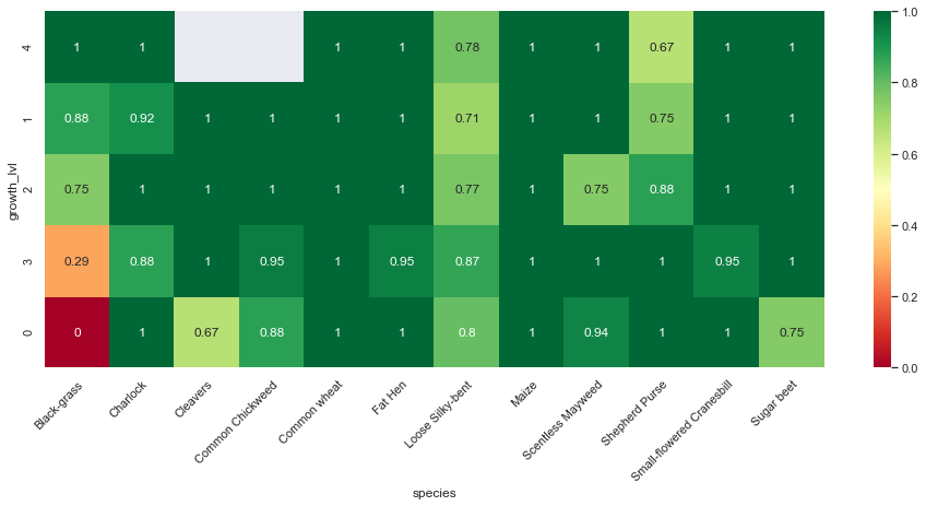
In addition to the confusion matrix per species, we can show how well our basic model performs per species and per growth stage.

# isolate train and test indexes as dataframe
df_X_train, df_X_test = train_test_split(resolution_df,
                                                    test_size=0.1,
                                                    random_state=seed,
                                                    stratify=resolution_df['species'])

# add predictions to dataframe
df_X_train.loc[:,'prediction'] = labels.classes_[y_train_pred]
df_X_test.loc[:,'prediction'] = labels.classes_[y_test_pred]

# define if prediction is correct
df_X_train['correct'] = df_X_train['species'] == df_X_train['prediction']
df_X_test['correct'] = df_X_test['species'] == df_X_test['prediction']

# group predictions by growth-phase and species
df_X_train = df_X_train.groupby(['growth_lvl', 'species'])['correct'].mean()
df_X_train = df_X_train.reset_index().pivot(index='growth_lvl', columns="species", values='correct')

df_X_test = df_X_test.groupby(['growth_lvl', 'species'])['correct'].mean()
df_X_test = df_X_test.reset_index().pivot(index='growth_lvl', columns="species", values='correct')

print("Training set:")
fig, ax = plt.subplots(figsize=(16,6))
sns.heatmap(df_X_train.reindex(CLUSTER_ORDER), ax=ax, cmap='RdYlGn', annot=True, annot_kws={"fontsize":12})
plt.setp(ax.get_xticklabels(), rotation=45, ha="right",rotation_mode="anchor")
ax.set_ylim
ax.set_ylim(0,5);

Training set:

print("Test set:")
fig, ax = plt.subplots(figsize=(16,6))
sns.heatmap(df_X_test.reindex(CLUSTER_ORDER), ax=ax, cmap='RdYlGn', annot=True, annot_kws={"fontsize":12})
plt.setp(ax.get_xticklabels(), rotation=45, ha="right",rotation_mode="anchor")
ax.set_ylim(0,5);

Test set:

Observations
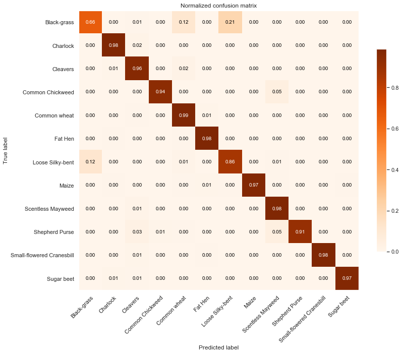
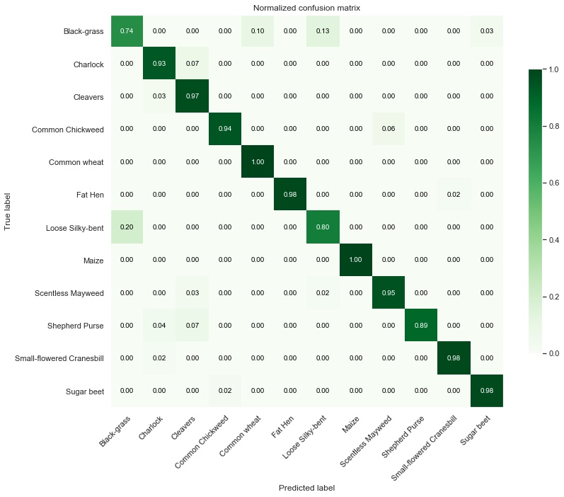
From the above confusion matrices and classification reports, we notice that our model performs well across all classes but two (Black-grass and Loose Silky-bent).

Indeed, the accuracy on these two classes are only 0.74 for the Black-grass and 0.80 for the Loose Silky-bent) on the validation set. We can also notice that these accuracies for the two class because the model mostly misclassifies Black-grass for Loose Silky-bent and vice-versa.

In addition, our model tends to do better on fully grown plants. Indeed, the high-resolution images (cluster 4) are almost all perfectly classified (except for the Loose Silky-Bent and the Shepeherd Purse).

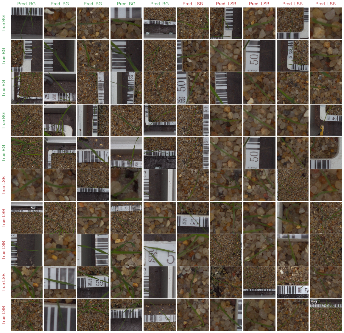
Let’s plot some of these errors against true specimens and assess if there is an apparent reason for the misclassifications.

# create a mapping between labels and classes
id_class_mapping = {idx: label for  idx, label in enumerate(labels.classes_)}
class_id_mapping = {label: idx for idx, label in id_class_mapping.items()}

# true Black-grass predicted as Loose Silky-bent
false_loose_silky = X_train[
    (y_train.argmax(axis=1) == class_id_mapping['Black-grass']) &
    (y_train_pred == class_id_mapping['Loose Silky-bent'])]

# true Loose Silky-bent predicted as Black-grass
false_black_grass = X_train[
    (y_train.argmax(axis=1) == class_id_mapping['Loose Silky-bent']) &
    (y_train_pred == class_id_mapping['Black-grass'])]

# true Loose Silky-bent correctly predicted
true_loose_silky = X_train[(y_train.argmax(axis=1) == y_train_pred) & (
    y_train_pred == class_id_mapping['Loose Silky-bent'])]

# true Black-grass correctly predicted
true_black_grass = X_train[(y_train.argmax(axis=1) == y_train_pred)
                           & (y_train_pred == class_id_mapping['Black-grass'])]

# create plot
fig, axes = plt.subplots(10, 10, figsize=(20, 20), gridspec_kw = {'wspace':0, 'hspace':0})
colors = ['grey', 'white']

for R in range(2):
    for C in range(2):

        # select set
        if R == 0 and C == 0:
            preds = true_black_grass
        elif R == 0 and C == 1:
            preds = false_loose_silky
        elif R == 1 and C == 0:
            preds = false_black_grass
        else:
            preds = true_loose_silky

        # randomly select images
        idxs = np.random.choice(preds.shape[0], 5 * 5)

        # true Black grass
        images = (preds[idxs, ...] * 255.).astype(np.uint8)

        for row in range(0 + 5 * R, 5 + 5 * R):
            for col in range(0 + 5 * C, 5 + 5 * C):
                image = images[(row - 5 * R) * 5 + (col - 5 * C)]
                #image = np.array(cv2.cvtColor(image, cv2.COLOR_BGR2RGB))

                axes[row, col].imshow(image)
                axes[row, col].grid(False)
                axes[row, col].set_xticklabels([])
                axes[row, col].set_yticklabels([])
                axes[row, col].set_aspect('equal')
                
                if row < 5 and col < 5:
                    title = "Pred. BG"
                    ct = 'g'
                    label = "True BG"
                    cl = 'g'
                elif row == 0 and col >= 5:
                    title = "Pred. LSB"
                    ct = 'r'
                    label = ""
                    cl = 'r'
                elif row >=5 and col == 0:
                    title = ""
                    label = "True LSB"
                    ct = 'r'
                    cl = 'r'
                else:
                    title = ""
                    label = ""
                    ct, cl = 'r', 'r'

                if row == 0:
                    axes[row, col].set_title(title, color = ct, fontsize = 15)
                if col == 0:
                    axes[row, col].set_ylabel(label, color = cl, fontsize = 15)

fig.subplots_adjust(hspace=0)
plt.show()

Observations
The above plot shows several examples of Black-grass and Loose silky-bent specimens both correctly and incorrectly classified. The main conclusion to draw from these observations is the that the model struggles to classify these two species because they are almost identical. Both of them can be described as thin and long green leaves similar to ordinary grass.

Before trying to adjust our model, we need to better understand our model and open the “black-box”. There are several model interpreters currently available. One of the popular one is LIME (Local Interpretable Model-Agnostic Explanations)

Model Inspection

fig, axes = plt.subplots(6, 4, figsize=(16, 30))

m = 0
for i in range(6):
    for j in range(4):

        # isolate species
        spec = np.arange(n_classes)[m//2]
        
        # find examples of the species
        idxes = y_train.argmax(axis=1) == spec
        
        # isolate image
        filtered_images = X_train[idxes,...]
        
        # random image
        image = filtered_images[np.random.randint(filtered_images.shape[0],size=1)[0],...]

        # make prediction
        test_pred = model.predict(image[np.newaxis,...], verbose=0).argmax(axis=1)
        
        # generate explanations
        explainer = lime_image.LimeImageExplainer(verbose=0)
        explanation = explainer.explain_instance(
            image,
            model.predict_proba,  # classification function
            top_labels=5,
            hide_color=0,
            num_samples=286)
        temp, mask = explanation.get_image_and_mask(explanation.top_labels[0],
                                                    positive_only=False,
                                                    num_features=5,
                                                    hide_rest=False)
        img_boundry1 = mark_boundaries(temp, mask)
                
        # convert label to species name
        predicted_species = id_class_mapping[test_pred[0]]
        
        # plot results
        axes[i, j].imshow(img_boundry1)
        axes[i, j].axis("off")
        axes[i, j].set_title("true " + id_class_mapping[spec] + "\n predicted: " +
                           predicted_species, fontsize=12)

        m += 1
plt.tight_layout()

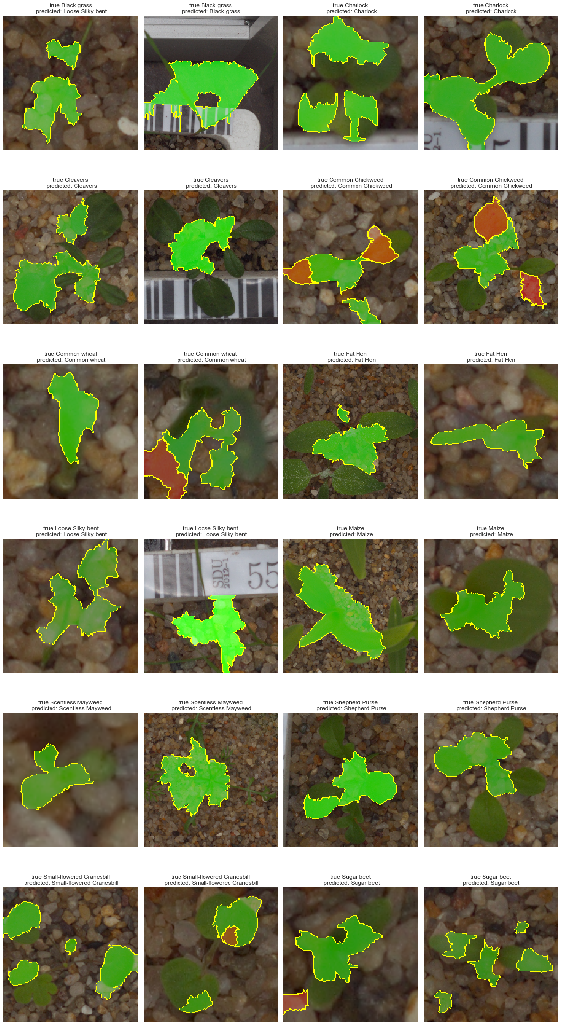
Observations

Although our model performs relatively well, we can see that in several cases shown above, the model uses the surrounding elements (pebbles, measuring label, and tags). The above plot shows areas leading to a positive predictions while red ones stands for negative impact on the predictions. We can see that the plant is often only partially used.

In conclusion, our model could be improved by removing extra components from the images.

Model Improvement

We have identified flaws in the predictions of our first model:

Uses external components to make predictions.
Struggles to make the difference between Black-grass and Loose Silky-bent

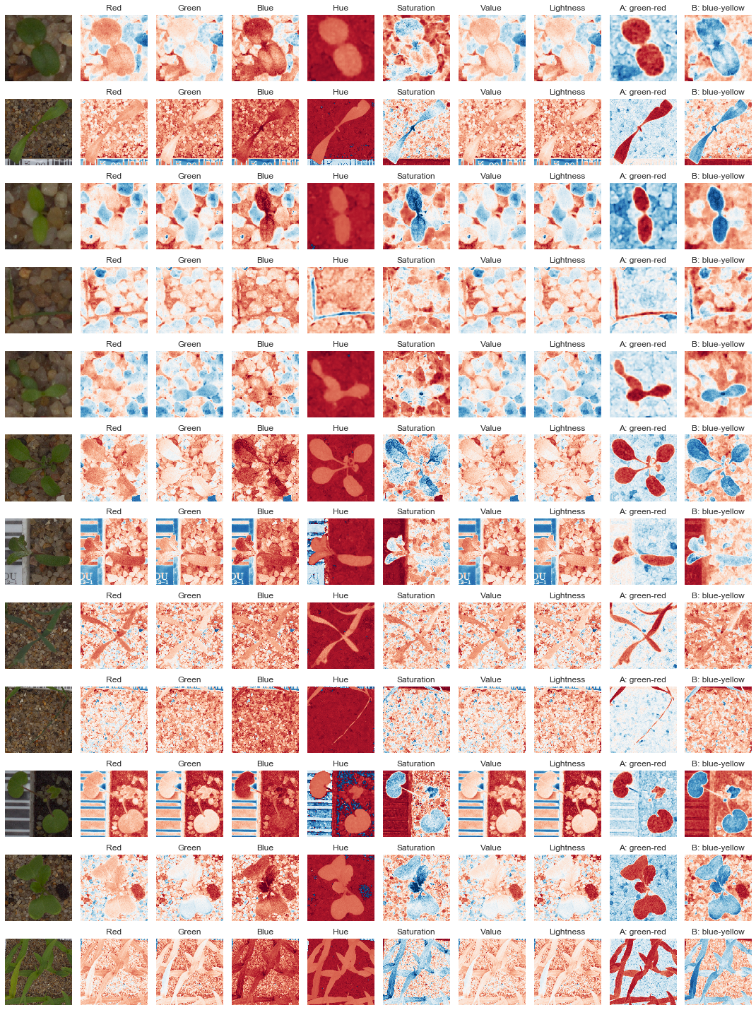
One of the main observations we can make is related to the photographs we have and the type of predictions. We could try to eliminate the surrounding components by focusing on the green channel of the image. Indeed, no element besides the seedling is green.

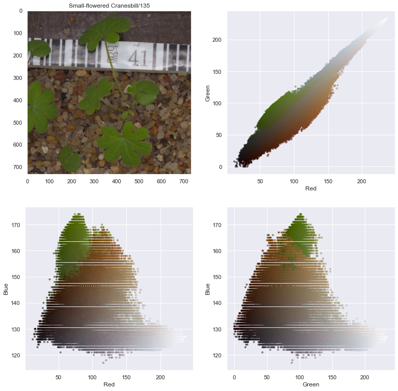
There are many different ways to represent images. The most common ones are RGB, HSV, and CIELAB. They are defined as follows.

Image Decomposition

RGB

Each image is encoded using three channels, this encoding is typically called RGB (Red, Blue, Green) corresponding to the magnitude of the color in each channel (from 0 to 255 as an 8 bit number). We can see if extracting specific channel can helps the seedling to stand out.

HSV (hue, saturation, value)

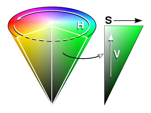
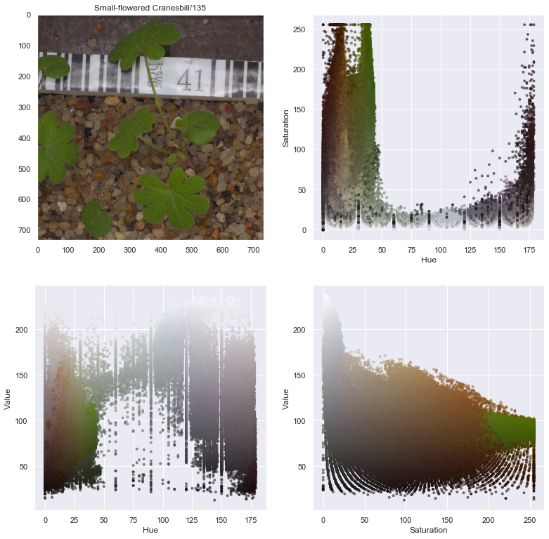
HSV is an alternative representation. The colors are encoded using 3 parameters:

Hue as an angle value 0° for red, 120° for green and 240° for blue.
Saturation is the intensity of the color as a number from 0 to 1 where 0 corresponds to the grayscale.
Value corresponds to the base grayscale value from 0 to 1 where 0 is black and 1 is white.

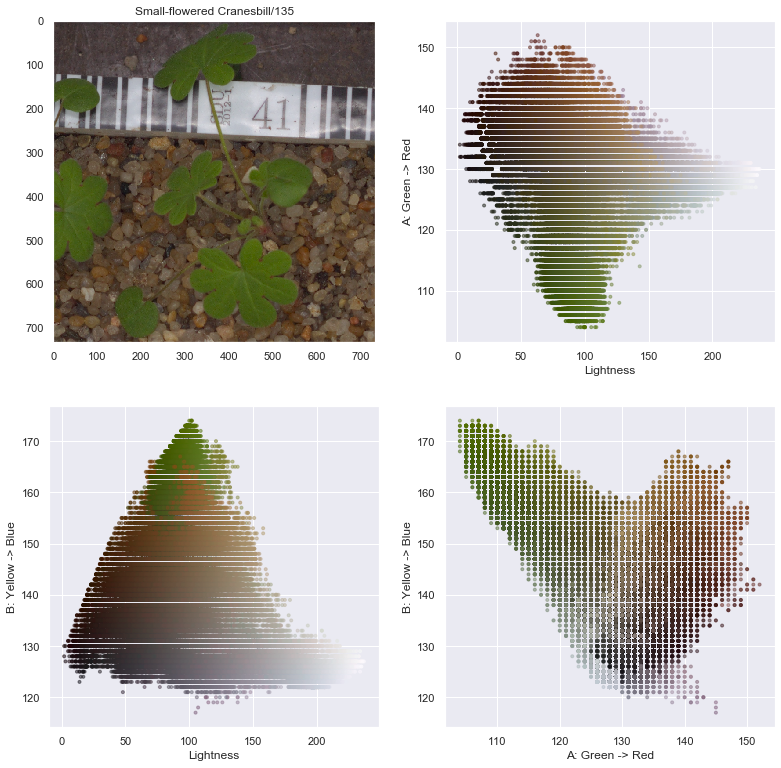
CIELAB

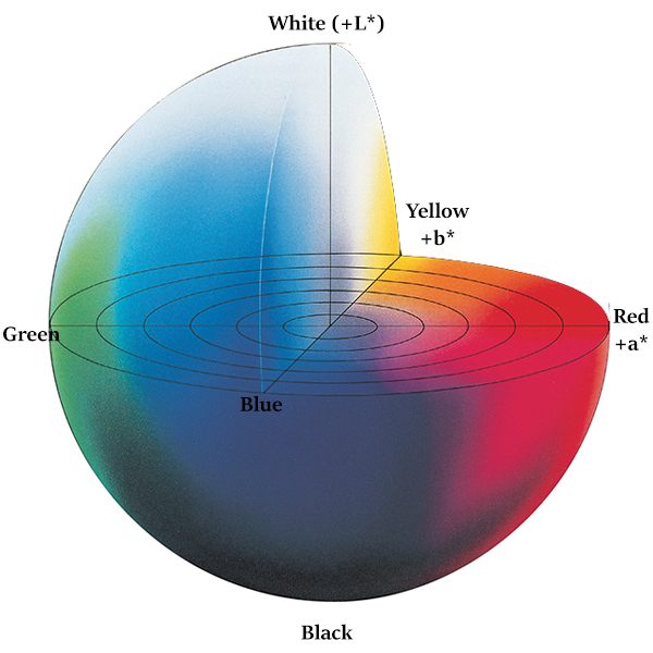
It expresses color as three values:

L* for the lightness from black (0) to white (100)
a* from green (−) to red (+)
b* from blue (−) to yellow (+)

# create plot
fig, axes = plt.subplots(12, 10, figsize=(15, 20))

titles = [ 
    'Red', 'Green', 'Blue',
    'Hue', 'Saturation', 'Value',
    'Lightness', 'A: green-red', 'B: blue-yellow'
]

for idx, plant in enumerate(resolution_df['species'].unique()):

    # isolate first cycle cutoff
    cutoff_num = cutoff_df.loc[cutoff_df['species'] ==
                               plant, 'drop'].values[0][0]

    # isolate file numbers less that cutoff_num
    all_file_nums = resolution_df.loc[(resolution_df['species'] == plant) & (
        resolution_df['file_num'] <= cutoff_num)].sort_values(
            by='file_num')['file_num']

    # select images at 50% of cycle
    selected_file_num = all_file_nums.quantile([0.5]).astype(int).values[0]
    image_rgb = imageio.imread(ZIPEXTRACT + plant + '/' + str(file_num) + '.png', as_gray=False, pilmode="RGB")
    image_hsv = matplotlib.colors.rgb_to_hsv(image_rgb)
    image_lab = color.rgb2lab(image_rgb)
    
    images = [image_rgb, image_hsv, image_lab]
    
    for k in range(10):
        if k==0:
                axes[idx,k].imshow(image_rgb)
                axes[idx,k].axis('off')

        else:
            image = images[(k-1)//3]
            axes[idx,k].imshow(image[:,:,(k-1)%3], cmap="RdBu")
            axes[idx,k].axis('off')
            axes[idx,k].set_title(titles[k-1], fontsize=12)
plt.tight_layout()

selected_image = resolution_df.iloc[4535]['full_path']
name = resolution_df.iloc[4535]['species'] + '/' + resolution_df.iloc[4535]['file_num'].astype(str)
name

'Small-flowered Cranesbill/135'

rgb = imageio.imread(selected_image, as_gray=False, pilmode="RGB")
hsv = cv2.cvtColor(rgb, cv2.COLOR_RGB2HSV)
lab = cv2.cvtColor(rgb, cv2.COLOR_RGB2LAB)

r, g, b = cv2.split(rgb)
h, s, v = cv2.split(hsv)
l, a, b = cv2.split(lab)

fig, axes = plt.subplots(2, 2, figsize=(13,13))

pixel_colors = rgb.reshape((np.shape(rgb)[0]*np.shape(rgb)[1], 3))
norm = colors.Normalize(vmin=-1.,vmax=1.)
norm.autoscale(pixel_colors)
pixel_colors = norm(pixel_colors).tolist()

axes[0,0].imshow(rgb)
axes[0,0].grid(False)
axes[0,0].set_title(name)

axes[0,1].scatter(r.flatten(), g.flatten(), facecolors=pixel_colors, marker=".", alpha=0.5)
axes[0,1].set_xlabel("Red")
axes[0,1].set_ylabel("Green")

axes[1,0].scatter(r.flatten(), b.flatten(), facecolors=pixel_colors, marker=".", alpha=0.5)
axes[1,0].set_xlabel("Red")
axes[1,0].set_ylabel("Blue")

axes[1,1].scatter(g.flatten(), b.flatten(), facecolors=pixel_colors, marker=".", alpha=0.5)
axes[1,1].set_xlabel("Green")
axes[1,1].set_ylabel("Blue")

plt.show()

fig, axes = plt.subplots(2, 2, figsize=(13,13))

pixel_colors = rgb.reshape((np.shape(rgb)[0]*np.shape(rgb)[1], 3))
norm = colors.Normalize(vmin=-1.,vmax=1.)
norm.autoscale(pixel_colors)
pixel_colors = norm(pixel_colors).tolist()

axes[0,0].imshow(rgb)
axes[0,0].grid(False)
axes[0,0].set_title(name)

axes[0,1].scatter(h.flatten(), s.flatten(), facecolors=pixel_colors, marker=".", alpha=0.5)
axes[0,1].set_xlabel("Hue")
axes[0,1].set_ylabel("Saturation")

axes[1,0].scatter(h.flatten(), v.flatten(), facecolors=pixel_colors, marker=".", alpha=0.5)
axes[1,0].set_xlabel("Hue")
axes[1,0].set_ylabel("Value")

axes[1,1].scatter(s.flatten(), v.flatten(), facecolors=pixel_colors, marker=".", alpha=0.5)
axes[1,1].set_xlabel("Saturation")
axes[1,1].set_ylabel("Value")

plt.show()

fig, axes = plt.subplots(2, 2, figsize=(13,13))

pixel_colors = rgb.reshape((np.shape(rgb)[0]*np.shape(rgb)[1], 3))
norm = colors.Normalize(vmin=-1.,vmax=1.)
norm.autoscale(pixel_colors)
pixel_colors = norm(pixel_colors).tolist()

axes[0,0].imshow(rgb)
axes[0,0].grid(False)
axes[0,0].set_title(name)

axes[0,1].scatter(l.flatten(), a.flatten(), facecolors=pixel_colors, marker=".", alpha=0.5)
axes[0,1].set_xlabel("Lightness")
axes[0,1].set_ylabel("A: Green -> Red")

axes[1,0].scatter(l.flatten(), b.flatten(), facecolors=pixel_colors, marker=".", alpha=0.5)
axes[1,0].set_xlabel("Lightness")
axes[1,0].set_ylabel("B: Yellow -> Blue")

axes[1,1].scatter(a.flatten(), b.flatten(), facecolors=pixel_colors, marker=".", alpha=0.5)
axes[1,1].set_xlabel("A: Green -> Red")
axes[1,1].set_ylabel("B: Yellow -> Blue")

plt.show()

Observations

From the above image decomposition plots, the Hue value of the HSV decomposition seems to be a good index to help decompose the seedling from the background. We can now implement a process to automatically remove background from images.

In order to properly remove the background, we can start by plotting the histogram of the Hue-level for sampled images. The plot below shows 5 samples of each species at different steps of the growth cycle with the histogram of the pixel hue.

# create plot
fig, axes = plt.subplots(24, 5, figsize=(15, 45))

for idx, plant in enumerate(resolution_df['species'].unique()):

    # isolate first cycle cutoff
    cutoff_num = cutoff_df.loc[cutoff_df['species'] ==
                               plant, 'drop'].values[0][0]

    # isolate file numbers less that cutoff_num
    all_file_nums = resolution_df.loc[(resolution_df['species'] == plant) & (
        resolution_df['file_num'] <= cutoff_num)].sort_values(
            by='file_num')['full_path']

    # select images at specific quantiles of cycle
    indexes = np.quantile(np.arange(0,all_file_nums.shape[0]),np.linspace(0,1,5), interpolation="lower")
    selected_file_paths = all_file_nums.values[indexes]

    # plot images
    for m, file_path in enumerate(selected_file_paths):
        image_rgb = imageio.imread(file_path,as_gray=False,pilmode="RGB")

        # plot image, hide grid, set title
        axes[idx*2, m].imshow(image_rgb)
        axes[idx*2, m].grid(False)
        axes[idx*2, m].set_title(plant + '/' + str(file_num))
        axes[idx*2, m].axis('off')
        
        # convert image to hue
        image_hsv = cv2.cvtColor(image_rgb, cv2.COLOR_RGB2HSV)
        sns.distplot(image_hsv[:, :, 0].flatten(),
                 ax=axes[idx*2+1,m],
                 kde=False, color="#4CB391", hist_kws={'alpha':1}, norm_hist=True)
plt.tight_layout()

Observations

From the above plots, it appears that the hue values of the pixels cluster into two groups. From there, we could consider two approaches:

Simple: define a threshold value of around 70 to manually divide the pixels into two cluster and eliminate the potion of the image where the hue of the pixels is larger than the threshold.
Complex but more suited to the various pixel distributions: for each image, cluster the hue of the pixels using a clustering algorithm and define the threshold as the boundary between the two clusters.

Since we want to reach the best accuracy possible, we will implement the clustering option.

def cluster_pixels_lab(image_rgb, return_labels=False, n_clusters=3):
    
    # convert image to hsv
    image_hsv = cv2.cvtColor(image_rgb, cv2.COLOR_RGB2HSV)
    
    # extract pixcels of Hue
    pixels = image_hsv[:,:,0].reshape(-1,1)
    
    # create and fit KMeans
    kmeans = KMeans(n_clusters=3, random_state=42, n_init=10).fit(pixels)
    
    # compute centers
    sorted_centers = np.sort(kmeans.cluster_centers_, axis=0)
    
    # corresponding clusters
    sorted_clusters = np.argsort(kmeans.cluster_centers_, axis=0)
    
    return image_hsv, sorted_centers.flatten(), sorted_clusters.flatten(), kmeans.labels_

fig, axes = plt.subplots(12, 2, figsize=(15, 45))
colors = ["royalblue", "gold", "silver", "lightgreen", "mediumpurple"]

for idx, plant in tqdm_notebook(enumerate(resolution_df['species'].unique())):

    # isolate first cycle cutoff
    cutoff_num = cutoff_df.loc[cutoff_df['species'] ==
                               plant, 'drop'].values[0][0]

    # isolate file numbers less that cutoff_num
    all_file_nums = resolution_df.loc[(resolution_df['species'] == plant) & (
        resolution_df['file_num'] <= cutoff_num)].sort_values(
            by='file_num')['full_path']

    # select images at specific quantiles of cycle
    indexes = np.quantile(np.arange(0, all_file_nums.shape[0]),
                          1.0,
                          interpolation="lower")
    file_path = all_file_nums.values[indexes]

    # read image
    image_rgb = imageio.imread(file_path, as_gray=False, pilmode="RGB")
    
    # plot image, hide grid, set title
    image_hsv, sorted_centers, sorted_clusters, labels = cluster_pixels_lab(image_rgb)
    
    axes[idx, 0].imshow(image_rgb)
    axes[idx, 0].grid(False)
    axes[idx, 0].set_title(plant + '/' + str(file_num))
    axes[idx, 0].axis('off')

    n, bins, patches = axes[idx, 1].hist(image_hsv[:, :, 0].flatten(),
                                         bins=30,
                                         alpha=0.0)
    
    for i, k in enumerate(sorted_clusters):
        color = cv2.cvtColor(np.uint8([[[sorted_centers[i],255,175]]]) , cv2.COLOR_HSV2RGB)/255.
        color = tuple(color[0][0].tolist())
        
        axes[idx, 1].hist(image_hsv[:,:,0].flatten()[labels==k],
                          bins=bins,
                          color=color,
                          label="Cluster " + str(k) + ', ' + "{:.2f}".format(sorted_centers[i]),
                          alpha=0.5)
    
        axes[idx, 1].axvline(sorted_centers[i], color=color, linestyle="--")
        axes[idx, 1].legend(loc='upper right')
plt.tight_layout();

HBox(children=(IntProgress(value=1, bar_style='info', max=1), HTML(value='')))

Observations

From above results depicting the pixel clustering, our approach is very promising.

In most cases, the green color is assigned a cluster. However, for cases where the seedling consists of grass-type leaves, a cluster cannot be assigned. However, we can use the information from the clustering of the other species to come up with a threshold.

# threshold to apply on A value
sensitivity = 25
colormin=(50-sensitivity,40,50)
colormax=(50+sensitivity,255,200)

def segment_plant(image_rgb):

    # apply blur
    blurr = cv2.GaussianBlur(image_rgb, (5, 5), 0)

    # convert to HSV
    image_hsv = cv2.cvtColor(blurr, cv2.COLOR_RGB2HSV)

    # apply filters
    mask = cv2.inRange(image_hsv, colormin, colormax)

    struc = cv2.getStructuringElement(cv2.MORPH_ELLIPSE, (11, 11))
    mask = cv2.morphologyEx(mask, cv2.MORPH_CLOSE, struc)

    # returned filtered image
    result = cv2.bitwise_and(image_rgb, image_rgb, mask=mask)
    return result, mask

scale_1 = 224
scale_2 = 70

fig, axes = plt.subplots(24, 5, figsize=(14, 50))
growth_cycles = ['Start', 'Full']

for idx, plant in enumerate(resolution_df['species'].unique()):

    # isolate first cycle cutoff
    cutoff_num = cutoff_df.loc[cutoff_df['species'] ==
                               plant, 'drop'].values[0][0]

    # isolate file numbers less that cutoff_num
    all_file_nums = resolution_df.loc[(resolution_df['species'] == plant) & (
        resolution_df['file_num'] <= cutoff_num)].sort_values(
            by='file_num')['full_path']

    # select images at specific quantiles of cycle
    indexes = np.quantile(np.arange(0, all_file_nums.shape[0]),
                          [0.0, 1.0],
                          interpolation="lower")
    file_paths = all_file_nums.values[indexes]

    i = 0
    for file_path in file_paths:
    
        image_rgb = imageio.imread(file_path,
                                       as_gray=False,
                                       pilmode="RGB")

        result, mask = segment_plant(image_rgb)
    
        reshape_1 = cv2.resize(result,(scale_1,scale_1))
        reshape_2 = cv2.resize(result,(scale_2,scale_2))
        
        axes[2*idx+i, 0].imshow(image_rgb)
        axes[2*idx+i, 1].imshow(mask)
        axes[2*idx+i, 2].imshow(result)
        axes[2*idx+i, 3].imshow(reshape_1)
        axes[2*idx+i, 4].imshow(reshape_2)
        axes[2*idx+i, 0].grid(False)
        axes[2*idx+i, 1].grid(False)
        axes[2*idx+i, 2].grid(False)
        axes[2*idx+i, 3].grid(False)
        axes[2*idx+i, 4].grid(False)
        axes[2*idx+i, 0].axis('off')
        axes[2*idx+i, 1].axis('off')
        axes[2*idx+i, 2].axis('off')
        axes[2*idx+i, 3].axis('off')
        axes[2*idx+i, 4].axis('off')
        
        axes[2*idx+i, 0].set_title(plant + '/Growth: ' + growth_cycles[i], fontsize=15)
        axes[2*idx+i, 1].set_title('Mask', fontsize=15)
        axes[2*idx+i, 2].set_title('Final, ({0},{1})'.format(*image_rgb.shape), fontsize=15)
        axes[2*idx+i, 3].set_title('Final, ({0},{1})'.format(*reshape_1.shape), fontsize=15)
        axes[2*idx+i, 4].set_title('Final, ({0},{1})'.format(*reshape_2.shape), fontsize=15)

        i+=1
plt.tight_layout();

Observations

Our image segmentation is now ready, the results look good with every species.

Generate New Images

We are going to segment each image and save it locally by using the same folder structure as the original dataset. Once the images have been segmented, we can feed them back into the model and train the CNN again.

SAVELOCATION = './DataAugmented_HSV_224/'

# create folder
if not os.path.exists(SAVELOCATION):
    os.makedirs(SAVELOCATION)

SCALE = 224

# extract image information
for folder in tqdm_notebook(listdir(ZIPEXTRACT), desc='1st loop'):

    # create folder
    if not os.path.exists(SAVELOCATION + folder):
        os.makedirs(SAVELOCATION + folder)

    for file in tqdm_notebook(listdir(ZIPEXTRACT + folder), desc='2nd loop'):

        # read image
        image_rgb = imageio.imread(ZIPEXTRACT + folder + '/' + file,
                               as_gray=False,
                               pilmode="RGB")

        # segment image
        masked_image, _ = segment_plant(image_rgb)

        # resize image
        resized_image = cv2.resize(masked_image, (SCALE, SCALE)) 
        
        # save image
        imageio.imwrite(SAVELOCATION + folder + '/' + file, resized_image)

# create full path to data
resolution_df['full_path_seg'] = SAVELOCATION + resolution_df[
    'species'] + '/' + resolution_df['file_name']
resolution_df.head()

	file_name	species	width	height	ratio	file_num	growth_lvl	full_path	full_path_seg
0	348.png	Cleavers	450.0	450.0	1.0	348	1	../Data/Cleavers/348.png	./DataAugmented_HSV_224/Cleavers/348.png
1	176.png	Cleavers	295.0	295.0	1.0	176	2	../Data/Cleavers/176.png	./DataAugmented_HSV_224/Cleavers/176.png
2	88.png	Cleavers	299.0	299.0	1.0	88	2	../Data/Cleavers/88.png	./DataAugmented_HSV_224/Cleavers/88.png
3	162.png	Cleavers	194.0	194.0	1.0	162	3	../Data/Cleavers/162.png	./DataAugmented_HSV_224/Cleavers/162.png
4	189.png	Cleavers	438.0	438.0	1.0	189	1	../Data/Cleavers/189.png	./DataAugmented_HSV_224/Cleavers/189.png

# batch size
batch_size = 32

# random seed
seed = 10

# load images into a numpy array
full_set_segm = []
for i in tqdm.notebook.tqdm(resolution_df['full_path_seg']):
    full_set_segm.append(imageio.imread(i,as_gray=False,pilmode="RGB"))
full_set_segm = np.asarray(full_set_segm)

print("{} images in full set.".format(full_set_segm.shape[0]))

HBox(children=(IntProgress(value=0, max=5539), HTML(value='')))

5539 images in full set.

# encode target
# create encoder and fit on training set
labels = LabelEncoder()
labels.fit(resolution_df['species'])

# display target classes
print('Classes'+str(labels.classes_))

# encode labels
encodedlabels = labels.transform(resolution_df['species'])
clearalllabels = np_utils.to_categorical(encodedlabels)

# store number of classes for future use
n_classes = clearalllabels.shape[1]

Classes['Black-grass' 'Charlock' 'Cleavers' 'Common Chickweed' 'Common wheat'
 'Fat Hen' 'Loose Silky-bent' 'Maize' 'Scentless Mayweed' 'Shepherd Purse'
 'Small-flowered Cranesbill' 'Sugar beet']

# scale data
full_set_segm = full_set_segm / 255.

# isolate train and test indexes
X_train, X_test, y_train, y_test = train_test_split(full_set_segm,
                                                    clearalllabels,
                                                    test_size=0.1,
                                                    random_state=seed,
                                                    stratify=resolution_df['species'])

# data augmentation
generator = ImageDataGenerator(rotation_range=180,
                               width_shift_range=0.1,
                               height_shift_range=0.1,
                               brightness_range=None,
                               shear_range=0.0,
                               zoom_range=0.1,
                               channel_shift_range=0.0,
                               fill_mode='nearest',
                               horizontal_flip=True,
                               vertical_flip=True,
                               dtype='float32')

np.random.seed(seed)

model = Sequential()

model.add(Conv2D(filters=32, kernel_size=(5, 5), input_shape=(SCALE, SCALE, 3), activation='relu'))
model.add(BatchNormalization(axis=3))
model.add(Conv2D(filters=64, kernel_size=(5, 5), activation='relu'))
model.add(MaxPooling2D((2, 2)))
model.add(BatchNormalization(axis=3))
model.add(Dropout(0.1))

model.add(Conv2D(filters=64, kernel_size=(5, 5), activation='relu'))
model.add(BatchNormalization(axis=3))
model.add(Conv2D(filters=64, kernel_size=(5, 5), activation='relu'))
model.add(MaxPooling2D((2, 2)))
model.add(BatchNormalization(axis=3))
model.add(Dropout(0.1))

model.add(Conv2D(filters=128, kernel_size=(5, 5), activation='relu'))
model.add(BatchNormalization(axis=3))
model.add(Conv2D(filters=128, kernel_size=(5, 5), activation='relu'))
model.add(MaxPooling2D((2, 2)))
model.add(BatchNormalization(axis=3))
model.add(Dropout(0.1))

model.add(Conv2D(filters=256, kernel_size=(5, 5), activation='relu'))
model.add(BatchNormalization(axis=3))
model.add(Conv2D(filters=256, kernel_size=(5, 5), activation='relu'))
model.add(MaxPooling2D((2, 2)))
model.add(BatchNormalization(axis=3))
model.add(Dropout(0.1))

model.add(Flatten())

model.add(Dense(256, activation='relu'))
model.add(BatchNormalization())
model.add(Dropout(0.5))

model.add(Dense(256, activation='relu'))
model.add(BatchNormalization())
model.add(Dropout(0.5))

model.add(Dense(n_classes, activation='softmax'))

# optimizer
optimizer = optimizers.Adam(lr=1e-2, beta_1=0.9, beta_2=0.999)

# define loss function
model.compile(optimizer=optimizer,
              loss=losses.categorical_crossentropy,
              metrics=['acc'])

# define optimization schedule with callbacks
lrate = ReduceLROnPlateau(monitor='val_acc',
                          factor=0.4,
                          patience=3,
                          verbose=1,
                          min_lr=0.00001)

if not os.path.exists("./Model_HSV_224"):
        os.makedirs("./Model_HSV_224")

filepath = "./Model_HSV_224/weights.best_{epoch:02d}-{val_acc:.2f}.hdf5"
checkpoints = ModelCheckpoint(filepath,
                              monitor='val_acc',
                              verbose=1,
                              save_best_only=False,
                              period=1)

callbacks_list = [lrate, checkpoints, TQDMNotebookCallback(leave_inner=False, leave_outer=True)]

model.summary()

Model: "sequential_2"
_________________________________________________________________
Layer (type)                 Output Shape              Param #   
=================================================================
conv2d_9 (Conv2D)            (None, 220, 220, 32)      2432      
_________________________________________________________________
batch_normalization_11 (Batc (None, 220, 220, 32)      128       
_________________________________________________________________
conv2d_10 (Conv2D)           (None, 216, 216, 64)      51264     
_________________________________________________________________
max_pooling2d_5 (MaxPooling2 (None, 108, 108, 64)      0         
_________________________________________________________________
batch_normalization_12 (Batc (None, 108, 108, 64)      256       
_________________________________________________________________
dropout_7 (Dropout)          (None, 108, 108, 64)      0         
_________________________________________________________________
conv2d_11 (Conv2D)           (None, 104, 104, 64)      102464    
_________________________________________________________________
batch_normalization_13 (Batc (None, 104, 104, 64)      256       
_________________________________________________________________
conv2d_12 (Conv2D)           (None, 100, 100, 64)      102464    
_________________________________________________________________
max_pooling2d_6 (MaxPooling2 (None, 50, 50, 64)        0         
_________________________________________________________________
batch_normalization_14 (Batc (None, 50, 50, 64)        256       
_________________________________________________________________
dropout_8 (Dropout)          (None, 50, 50, 64)        0         
_________________________________________________________________
conv2d_13 (Conv2D)           (None, 46, 46, 128)       204928    
_________________________________________________________________
batch_normalization_15 (Batc (None, 46, 46, 128)       512       
_________________________________________________________________
conv2d_14 (Conv2D)           (None, 42, 42, 128)       409728    
_________________________________________________________________
max_pooling2d_7 (MaxPooling2 (None, 21, 21, 128)       0         
_________________________________________________________________
batch_normalization_16 (Batc (None, 21, 21, 128)       512       
_________________________________________________________________
dropout_9 (Dropout)          (None, 21, 21, 128)       0         
_________________________________________________________________
conv2d_15 (Conv2D)           (None, 17, 17, 256)       819456    
_________________________________________________________________
batch_normalization_17 (Batc (None, 17, 17, 256)       1024      
_________________________________________________________________
conv2d_16 (Conv2D)           (None, 13, 13, 256)       1638656   
_________________________________________________________________
max_pooling2d_8 (MaxPooling2 (None, 6, 6, 256)         0         
_________________________________________________________________
batch_normalization_18 (Batc (None, 6, 6, 256)         1024      
_________________________________________________________________
dropout_10 (Dropout)         (None, 6, 6, 256)         0         
_________________________________________________________________
flatten_2 (Flatten)          (None, 9216)              0         
_________________________________________________________________
dense_4 (Dense)              (None, 256)               2359552   
_________________________________________________________________
batch_normalization_19 (Batc (None, 256)               1024      
_________________________________________________________________
dropout_11 (Dropout)         (None, 256)               0         
_________________________________________________________________
dense_5 (Dense)              (None, 256)               65792     
_________________________________________________________________
batch_normalization_20 (Batc (None, 256)               1024      
_________________________________________________________________
dropout_12 (Dropout)         (None, 256)               0         
_________________________________________________________________
dense_6 (Dense)              (None, 12)                3084      
=================================================================
Total params: 5,765,836
Trainable params: 5,762,828
Non-trainable params: 3,008
_________________________________________________________________

# Fit the model
history = model.fit_generator(generator.flow(X_train, y_train, batch_size=batch_size),
                    epochs=50,
                    steps_per_epoch=np.ceil(X_train.shape[0] / batch_size),
                    validation_data=(X_test, y_test),
                    callbacks=callbacks_list,
                    verbose=2)

Epoch 1/50 - 2341s - loss: 2.2011 - acc: 0.3446 - val_loss: 7.5625 - val_acc: 0.0776  
Epoch 00001: saving model to ./Model_HSV_224/weights.best_01-0.08.hdf5  
Epoch 2/50 - 2088s - loss: 1.4293 - acc: 0.5153 - val_loss: 4.6444 - val_acc: 0.1498  
Epoch 00002: saving model to ./Model_HSV_224/weights.best_02-0.15.hdf5  
Epoch 3/50 - 2077s - loss: 1.1777 - acc: 0.5972 - val_loss: 4.0929 - val_acc: 0.3159  
Epoch 00003: saving model to ./Model_HSV_224/weights.best_03-0.32.hdf5  
.  
.  
.  
Epoch 47/50 - 1931s - loss: 0.1805 - acc: 0.9336 - val_loss: 0.2560 - val_acc: 0.9043  
Epoch 00047: saving model to ./Model_HSV_224/weights.best_47-0.90.hdf5  
Epoch 48/50 - 1947s - loss: 0.1959 - acc: 0.9316 - val_loss: 0.2534 - val_acc: 0.9043  
Epoch 00048: saving model to ./Model_HSV_224/weights.best_48-0.90.hdf5  
Epoch 49/50 - 1947s - loss: 0.1805 - acc: 0.9334 - val_loss: 0.2516 - val_acc: 0.9061  
Epoch 00049: saving model to ./Model_HSV_224/weights.best_49-0.91.hdf5  
Epoch 50/50 - 1947s - loss: 0.1810 - acc: 0.9374 - val_loss: 0.2566 - val_acc: 0.9061  
Epoch 00050: saving model to ./Model_HSV_224/weights.best_50-0.91.hdf5

lr = pd.read_csv('lr_HSV.csv', index_col=0)
history = pd.read_csv('history_HSV.csv', index_col=0)

fig, axes = plt.subplots(2, 2, figsize=(16, 12))
axes[0,0].plot(history['loss'], label='training', c='dodgerblue')
axes[0,0].plot(history['val_loss'], label='validation', c='crimson')
axes[0,0].legend()
axes[0,0].set_title("Loss function", fontsize=15)
axes[0,0].set_xlabel("epochs")
axes[0,0].set_ylabel("loss")

axes[0,1].plot(history['acc'], label='training', c='dodgerblue')
axes[0,1].plot(history['val_acc'], label='validation', c='crimson')
axes[0,1].legend()
axes[0,1].set_title("Accuracy", fontsize=15)
axes[0,1].set_xlabel("epochs")
axes[0,1].set_ylabel("accuracy")

axes[1,0].plot(lr['lr'], c='dodgerblue')
axes[1,0].set_title("Learning Rate", fontsize=15)
axes[1,0].set_xlabel("epochs")
axes[1,0].set_ylabel("learning rate")
axes[1,0].set_ylim(0,0.011)

axes[-1,-1].axis('off');

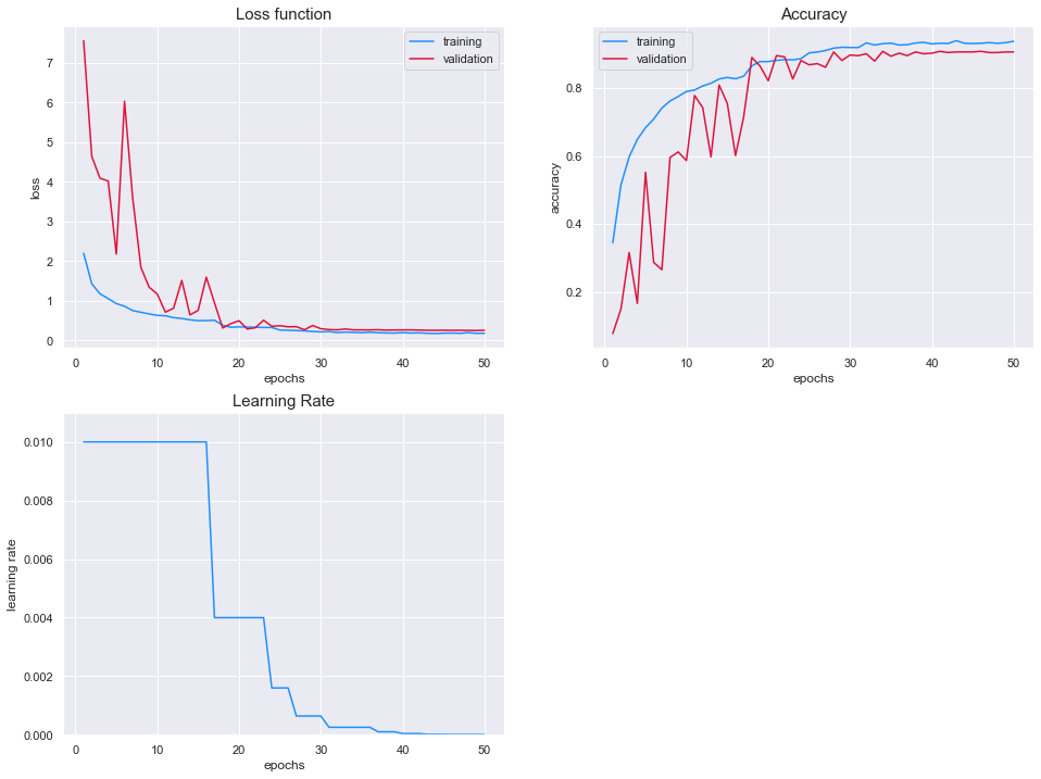
Results

The value of the loss functions is almost identical between the two sets once the training has stabilized. We can see that the model has reached a stable configuration as the loss function of the training set and test set both plateau after 30 epochs.

In addition, the accuracy of both models reach around 90%. Our initial model reached 92% accuracy on the test set. However, we saw that the model was using leakage by leverage information located in the periphery of the seedling.

Predictions and Results

print("Maximum accuray on validation step:")
print(" Epoch: {}".format(np.argmax(history['val_acc'])))
print("        {:.2f}%".format(history['val_acc'].values.max()*100))

Maximum accuray on validation step:
 Epoch: 34
        90.79%

We now load the model weights corresponding to the best accuracy on the test set.

# load best model
model.load_weights("./Model_HSV_224/weights.best_34-0.91.hdf5")

We now make predictions on the train and test sets.

y_train_pred = model.predict(X_train, verbose=1).argmax(axis=1)
y_test_pred = model.predict(X_test, verbose=1).argmax(axis=1)

4985/4985 [==============================] - 779s 156ms/step
554/554 [==============================] - 81s 146ms/step

Similar to the first model, we can plot the confusion matrices for both the training and test sets.

print('Training Data')
ax = TAD_tools_v01.plot_confusion_matrix(y_train.argmax(axis=1),
                                    y_train_pred,
                                    labels.classes_,
                                    normalize=True,
                                    title=None,
                                    cmap=plt.cm.Oranges,
                                    figsize=(12,12))

ax.set_ylim(11.5,-0.5);

Training Data

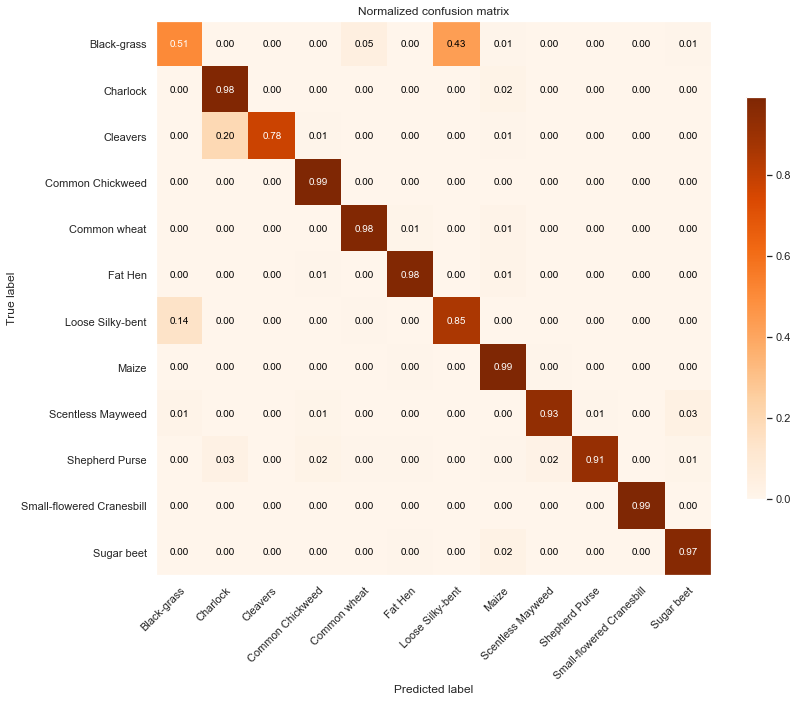
print('Test Data')
ax = TAD_tools_v01.plot_confusion_matrix(y_test.argmax(axis=1),
                                    y_test_pred,
                                    labels.classes_,
                                    normalize=True,
                                    title=None,
                                    cmap=plt.cm.Greens,
                                    figsize=(12,12))

ax.set_ylim(11.5,-0.5);

Test Data

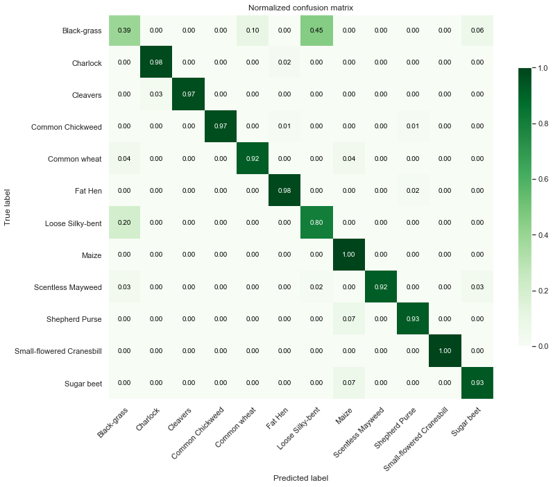
Observations

From the above, we can clearly see that our model has lost some accuracy on the Black-grass class. The class accuracy is not only 0.51 and 0.39 for the training and test sets respectively. However, the model has improved its predictions on the other classes.

print("Accurancy:")
print("   Train: {:.2f}%".format(metrics.accuracy_score(y_train.argmax(axis=1), y_train_pred)*100))
print("   Test:  {:.2f}%".format(metrics.accuracy_score(y_test.argmax(axis=1), y_test_pred)*100))

print("\nF1-score")
print("   Train: {:.3f}%".format(metrics.f1_score(y_train.argmax(axis=1), y_train_pred, average='weighted')*100))
print("   Test:  {:.3f}%".format(metrics.f1_score(y_test.argmax(axis=1), y_test_pred, average='weighted')*100))

print("\nClassification Report")
print(metrics.classification_report(y_train.argmax(axis=1), y_train_pred))
print(metrics.classification_report(y_test.argmax(axis=1), y_test_pred))

Accurancy:
   Train: 91.65%
   Test:  90.79%

F1-score
   Train: 91.536%
   Test:  90.790%

Classification Report
              precision    recall  f1-score   support

           0       0.57      0.51      0.54       278
           1       0.86      0.98      0.91       407
           2       1.00      0.78      0.87       301
           3       0.98      0.99      0.98       642
           4       0.91      0.98      0.94       228
           5       0.98      0.98      0.98       484
           6       0.82      0.85      0.84       686
           7       0.87      0.99      0.93       231
           8       0.99      0.93      0.96       546
           9       0.98      0.91      0.95       247
          10       1.00      0.99      0.99       518
          11       0.94      0.97      0.95       417

    accuracy                           0.92      4985
   macro avg       0.91      0.90      0.90      4985
weighted avg       0.92      0.92      0.92      4985

              precision    recall  f1-score   support

           0       0.40      0.39      0.39        31
           1       0.98      0.98      0.98        45
           2       1.00      0.97      0.99        34
           3       1.00      0.97      0.99        71
           4       0.88      0.92      0.90        25
           5       0.96      0.98      0.97        54
           6       0.80      0.80      0.80        76
           7       0.81      1.00      0.90        26
           8       1.00      0.92      0.96        61
           9       0.93      0.93      0.93        27
          10       1.00      1.00      1.00        58
          11       0.91      0.93      0.92        46

    accuracy                           0.91       554
   macro avg       0.89      0.90      0.89       554
weighted avg       0.91      0.91      0.91       554

# isolate train and test indexes as dataframe
df_X_train, df_X_test = train_test_split(resolution_df,
                                                    test_size=0.1,
                                                    random_state=seed,
                                                    stratify=resolution_df['species'])

# add predictions to dataframe
df_X_train.loc[:,'prediction_HSV'] = labels.classes_[y_train_pred]
df_X_test.loc[:,'prediction_HSV'] = labels.classes_[y_test_pred]

# define if prediction is correct
df_X_train['correct'] = df_X_train['species'] == df_X_train['prediction_HSV']
df_X_test['correct'] = df_X_test['species'] == df_X_test['prediction_HSV']

# group predictions by growth-phase and species
df_X_train = df_X_train.groupby(['growth_lvl', 'species'])['correct'].mean()
df_X_train = df_X_train.reset_index().pivot(index='growth_lvl', columns="species", values='correct')

df_X_test = df_X_test.groupby(['growth_lvl', 'species'])['correct'].mean()
df_X_test = df_X_test.reset_index().pivot(index='growth_lvl', columns="species", values='correct')

print("Training set:")
fig, ax = plt.subplots(figsize=(16,6))
sns.heatmap(df_X_train.reindex(CLUSTER_ORDER), ax=ax, cmap='RdYlGn', annot=True, annot_kws={"fontsize":12}, vmin=0)
plt.setp(ax.get_xticklabels(), rotation=45, ha="right",rotation_mode="anchor")
ax.set_ylim
ax.set_ylim(0,5);

Training set:

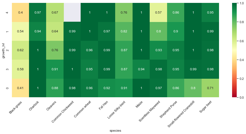
print("Test set:")
fig, ax = plt.subplots(figsize=(16,6))
sns.heatmap(df_X_test.reindex(CLUSTER_ORDER), ax=ax, cmap='RdYlGn', annot=True, annot_kws={"fontsize":12}, vmin=0)
plt.setp(ax.get_xticklabels(), rotation=45, ha="right",rotation_mode="anchor")
ax.set_ylim(0,5);

Test set:

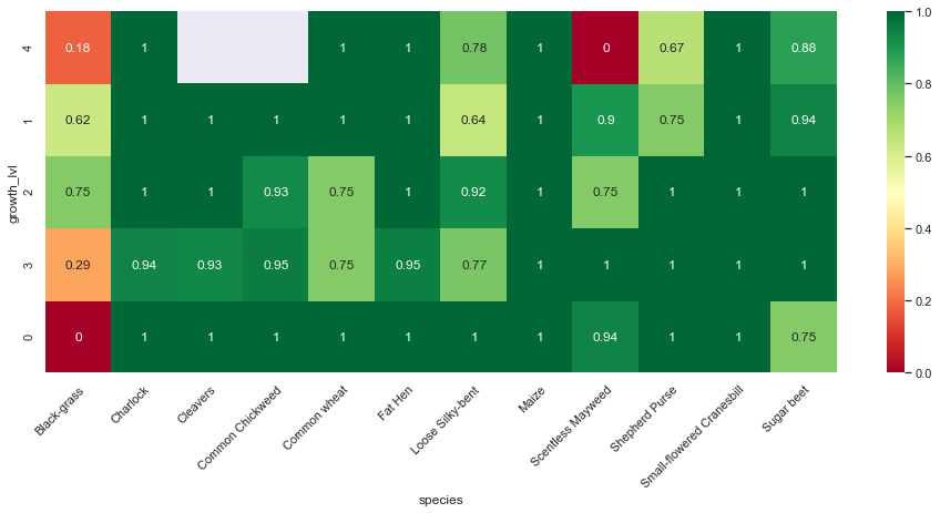
Final Model Inspection

fig, axes = plt.subplots(6, 4, figsize=(16, 30))

m = 0
for i in range(6):
    for j in range(4):

        # isolate species
        spec = np.arange(n_classes)[m//2]
        
        # find examples of the species
        idxes = y_train.argmax(axis=1) == spec
        
        # isolate image
        filtered_images = X_train[idxes,...]
        
        # random image
        image = filtered_images[np.random.randint(filtered_images.shape[0],size=1)[0],...]

        # make prediction
        test_pred = model.predict(image[np.newaxis,...], verbose=0).argmax(axis=1)
        
        # generate explanations
        explainer = lime_image.LimeImageExplainer(verbose=0)
        explanation = explainer.explain_instance(
            image,
            model.predict_proba,  # classification function
            top_labels=5,
            hide_color=0,
            num_samples=286)
        temp, mask = explanation.get_image_and_mask(explanation.top_labels[0],
                                                    positive_only=False,
                                                    num_features=5,
                                                    hide_rest=False)
        img_boundry1 = mark_boundaries(temp, mask)
                
        # convert label to species name
        predicted_species = id_class_mapping[test_pred[0]]
        
        # plot results
        axes[i, j].imshow(img_boundry1)
        axes[i, j].axis("off")
        axes[i, j].set_title("true " + id_class_mapping[spec] + "\n predicted: " +
                           predicted_species, fontsize=12)

        m += 1
plt.tight_layout()

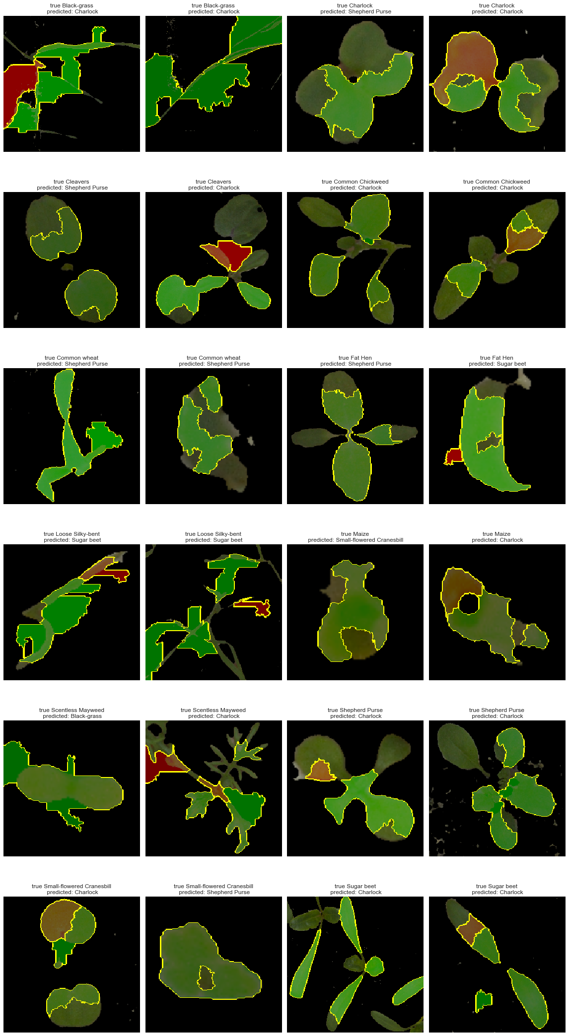
Conclusion

In conclusion, we were able to produce a model relying only on the shape, size, and colors of the seedlings. This model is capable of making correct predictions more than 90% of the times on 12 different seedling species. If we were to improve this model and its data collection, the following recommendations would be proposed:

Standardize photographs by taking pictures from the same distance, same focus.
Build a model to classify the Loose-Silky bent and Black-grass together then develop a model specifically to classify these two species.
Collect information regarding the importance of misclassification of certain species. Weights can then be incorporated in the model.