Art Style Predictions

Goal
The available dataset consists of all the paintings and artworks from Wikiart.
The objective is to build a model able to predict the style of an uploaded image amongst the top 18 most popular styles.
My main objective through this project was to build and deploy a model and an associated API.
The python code is available in my Github repository.
For the deployment of this model, I have chosen the following:
- Build a flask app to create a web interface.
- Host some of the data into a MongoDB database.
- Deploy a live version using an AWS instance (EC2+S3).
API
Deployed API
A live version can be accessed HERE.
Architecture
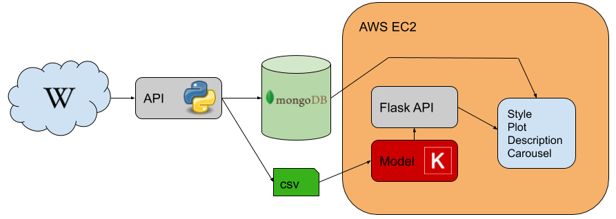
The application is built using:
- Wikiart Web Scraper (Repository)
- MongoDB database containing meta information about every artwork
- Keras models
- Flask API
- The application is stored on Amazon S3
- The instance of the application is hosted on an Ubuntu 18.04 server (Amazon EC2)
Interface
Data
Keras can use the directory structure to determine the image classes. To do so, we need to store each image into a folder titled with the painting style. A python function organize_directories in module models.py is used to move each picture in its corresponding style directory. Note that the images are also resized as 224x224x3 and saved as png. Finally, the distribution is done by splitting the dataset into a train and test sets. The split is done by stratifying the styles and assigning randomly 20% of each styles into the test set.
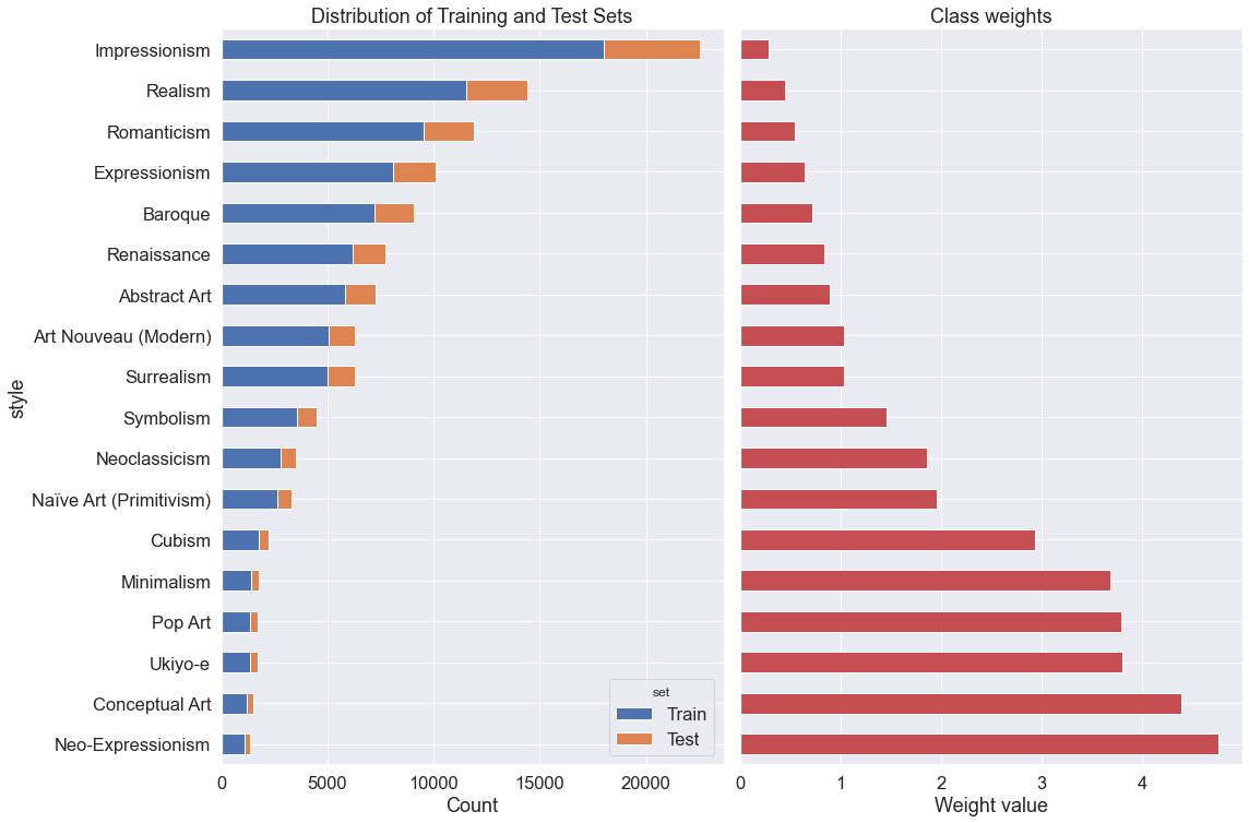
As shown above, the dataset has been divided into the train and test set while maintaining the class proportion. In order to avoid bias over class that are overly represented (Impressionism, Realism…). The metrics of interest will be weighted so that each class is assigned the same importance.
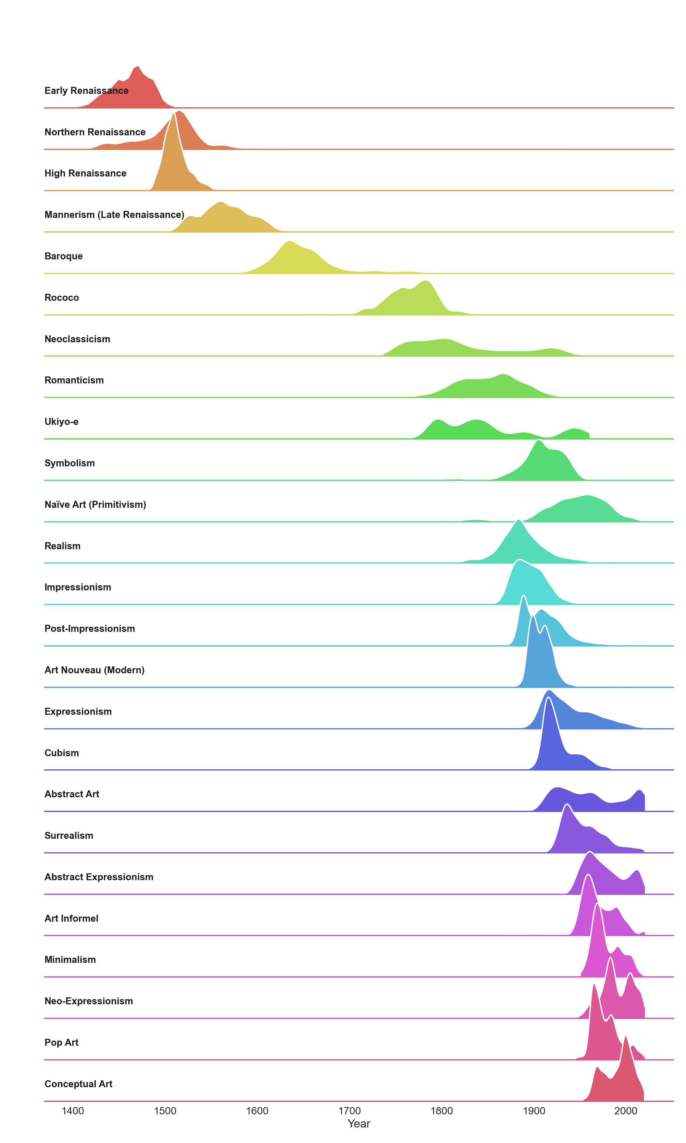
Model
Convolutional Neural Network
In this section, we will train a CNN to predict the species feature. The approach is divided between the following steps:
- Encode the target feature
- Download the data
- Split the data between a training and test set
- Perform data augmentation
- Determine the cost function to be optimized
- Data Loader, Validation and Data Augmentation
In order for our model to generalize well on unseen data, a good practice consists of using image transformation to create new unseen examples. We need to ensure that our model does not over fit the training data. To do so, we are using a training set and a test set both taken from the original dataset.
Keras contains useful tools to help process image files and feed them in batches to the model. We will be using a generator for both the train and test phases.
First, we must create a new feature to our dataset which contains the full path to each image. Then, we can create two generators, the training generator will contains several data augmentation transformation (horizontal and vertical flips, zoom). Both the train and test generator will normalize the pixel values. Finally, the images will be sent to the model using batches of 16 RGB images reshaped at 224x224.
Transfer Learning - First Generation
Before we train a model on the entire dataset, we need to investigate the following modeling choices:
- Architecture
- Optimization metrics
- Callbacks
- Optimizers
During this initial phase, we will test 5 different base models using only 1,000 images per class. The considered base models are:
- ResNet50
- Inception V3
- MobileNet V2
- Xception
- VGG16
For each model, we remove the top layer and add a custom model to it. This top model is defined as follows:
- Conv2D (512, 2, relu)
- Flatten
- Dense (2048, relu)
- Dense (1024, relu)
- Dense (512, relu)
- Dense (256, relu)
- Dense (64, relu)
- Dense (18, softmax)
## load results
results = pd.read_csv('../data/training_phase1.csv')
results['size_total_MB'] = results['size_base_MB'] + results['size_top_MB']
results
| model | tag | val_loss | val_accuracy | loss | accuracy | size_base_MB | size_top_MB | size_total_MB | |
|---|---|---|---|---|---|---|---|---|---|
| 0 | 1.a.1000 | ResNet50 | 2.512670 | 0.208333 | 2.610792 | 0.181167 | 94.7 | 131.6 | 226.3 |
| 1 | 1.b.1000 | VGG16 | 1.930195 | 0.373611 | 1.895698 | 0.385111 | 58.9 | 106.5 | 165.4 |
| 2 | 1.c.1000 | InceptionV3 | 1.890462 | 0.391667 | 1.687830 | 0.453889 | 87.9 | 89.7 | 177.6 |
| 3 | 1.d.1000 | MobileNetV2 | 1.745986 | 0.436389 | 1.514181 | 0.501667 | 9.4 | 119.0 | 128.4 |
| 4 | 1.e.1000 | Xception | 1.799670 | 0.419722 | 1.740675 | 0.439667 | 83.7 | 131.6 | 215.3 |
%matplotlib inline
fig, ax = plt.subplots(figsize=(8,6))
results[['tag', 'val_accuracy', 'accuracy']].set_index('tag').plot(ax=ax, kind='barh', color=['b','r'])
ax.set_title("Model Accuracy")
ax.set_xlabel('Accuracy')
plt.show();
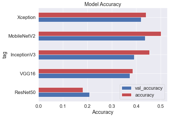
The MobileNet V2 seems to be the best choice, it scores the highest in term of validation accuracy and is also the lightest model (128M). However, this weight is still a bit much to easily deploy on a Heroku instance. We make a new version of the top model by decreasing the size of the top model first dense layer from 2048 neurons to 1024.
Transfer Learning - Second Generation
Architecture - MobileNet V2
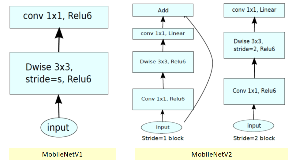
- There are 3 layers for both types of blocks.
- The first layer is 1×1 convolution with ReLU6.
- The second layer is the depthwise convolution.
- The third layer is another 1×1 convolution but without any non-linearity. It is claimed that if ReLU is used again, the deep networks only have the power of a linear classifier on the non-zero volume part of the output domain.

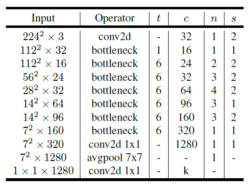
where:
- t: expansion factor
- c: number of output channels
- n: repeating number
- s: stride.
- 3×3 kernels are used for spatial convolution.
This top model is defined as follows:
- Conv2D (512, 2, relu)
- Flatten
- Dense (1024, relu)
- Dense (1024, relu)
- Dense (512, relu)
- Dense (256, relu)
- Dense (64, relu)
- Dense (18, softmax)
Results
Training
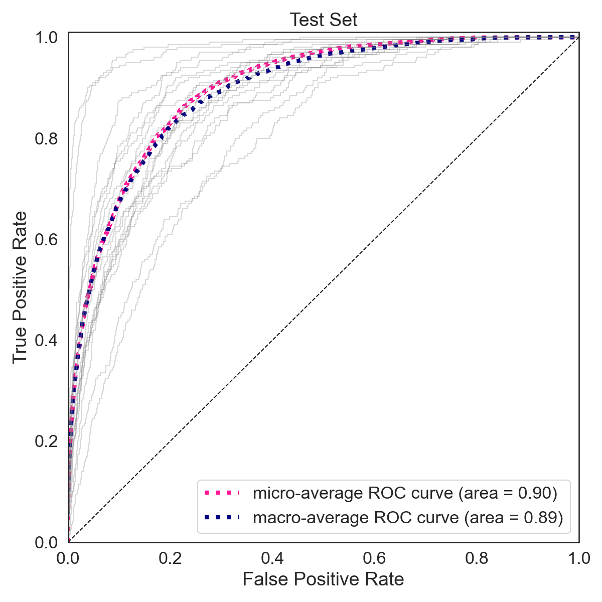
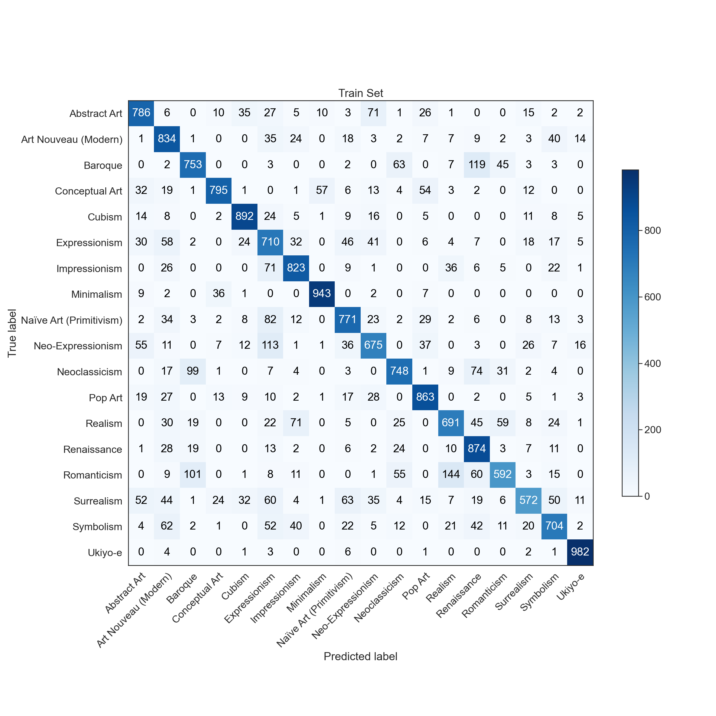
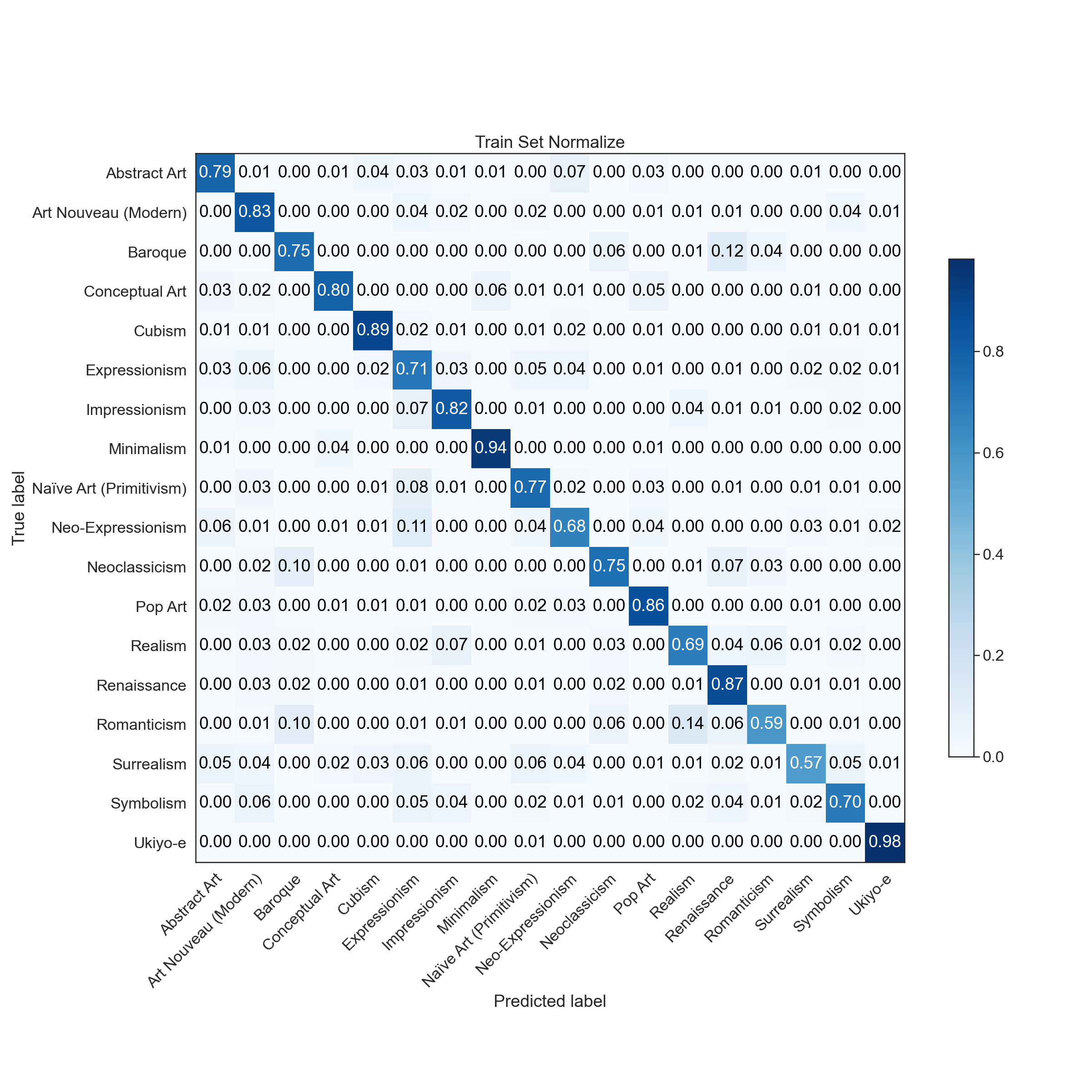
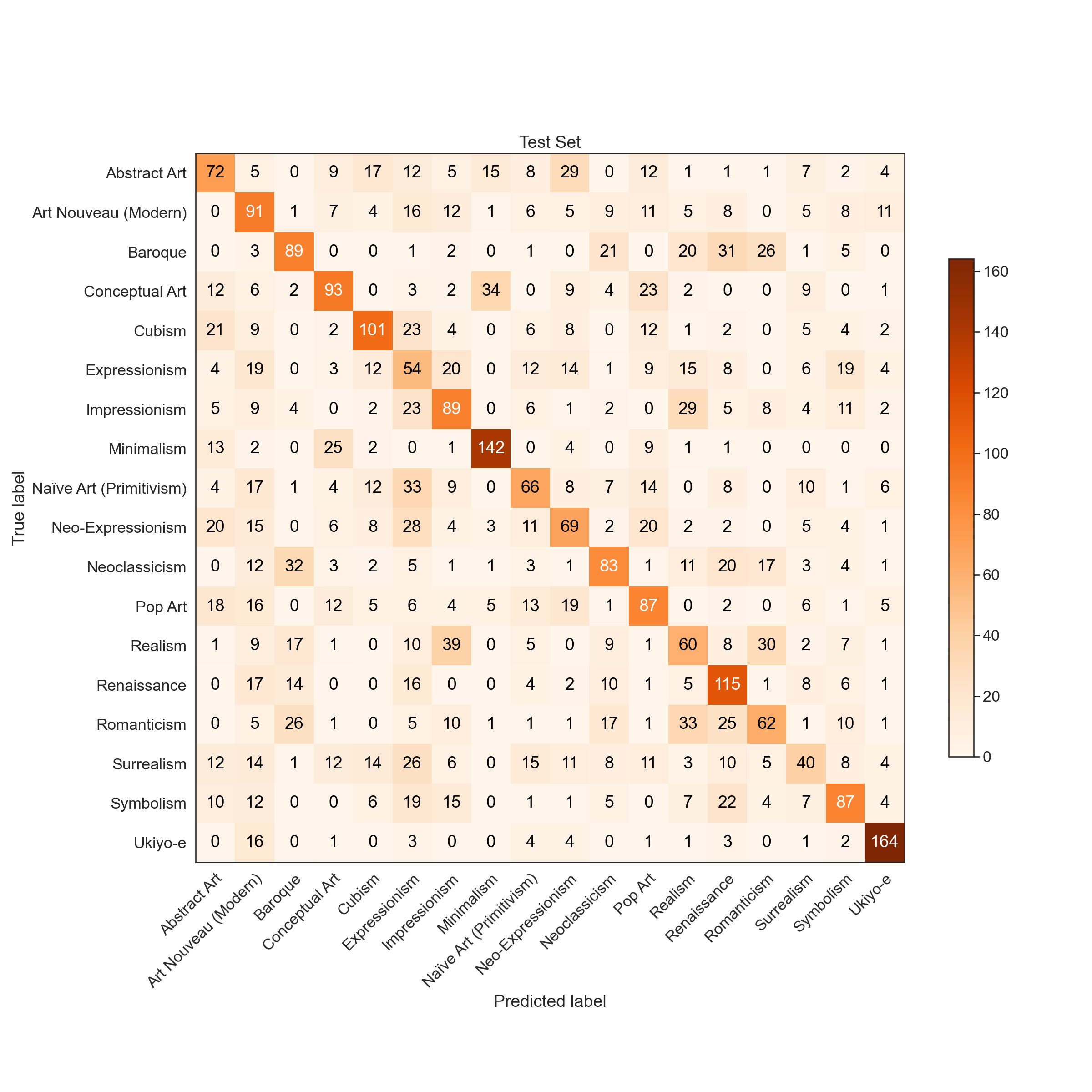
As shown below the training accuracy plateaus at 56% (benchmark accuracy is 5.6%) while the accuracy on the test set is 43%.
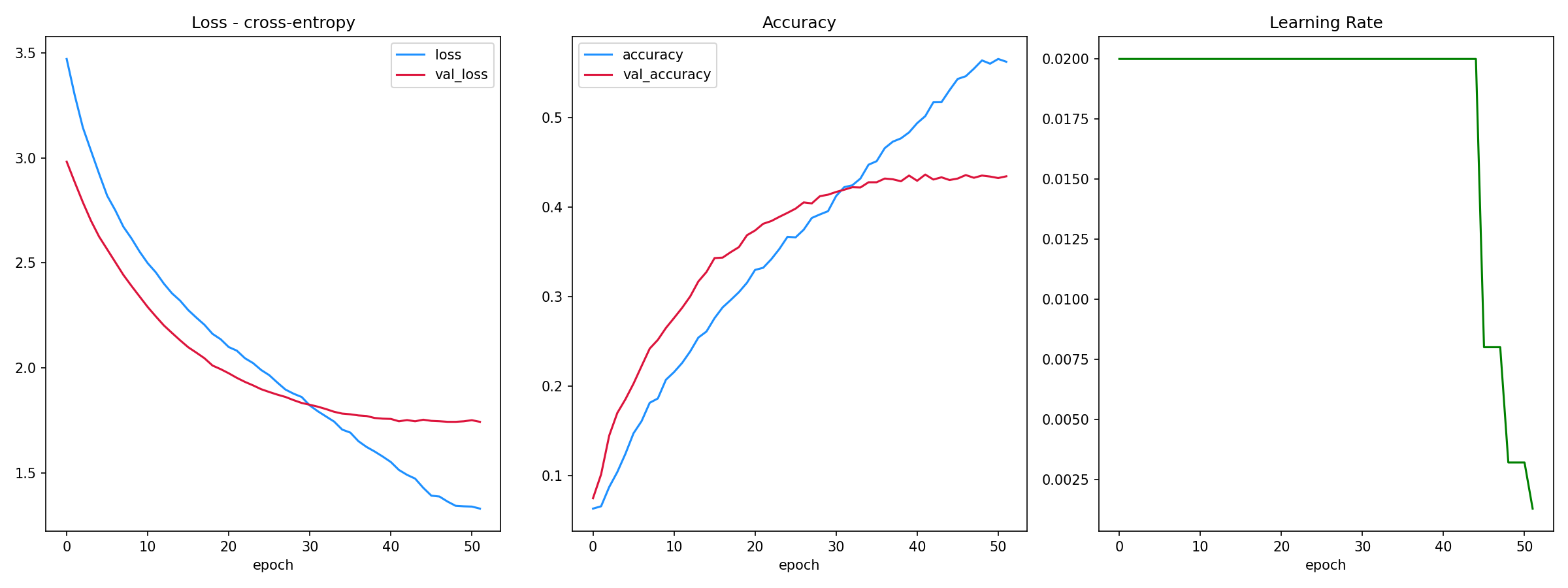
The F-1 score on the training set is 0.78 (macro average) and 0.78 (weighted average). The F-1 score on the training set is 0.43 (macro average) and 0.44 (weighted average).
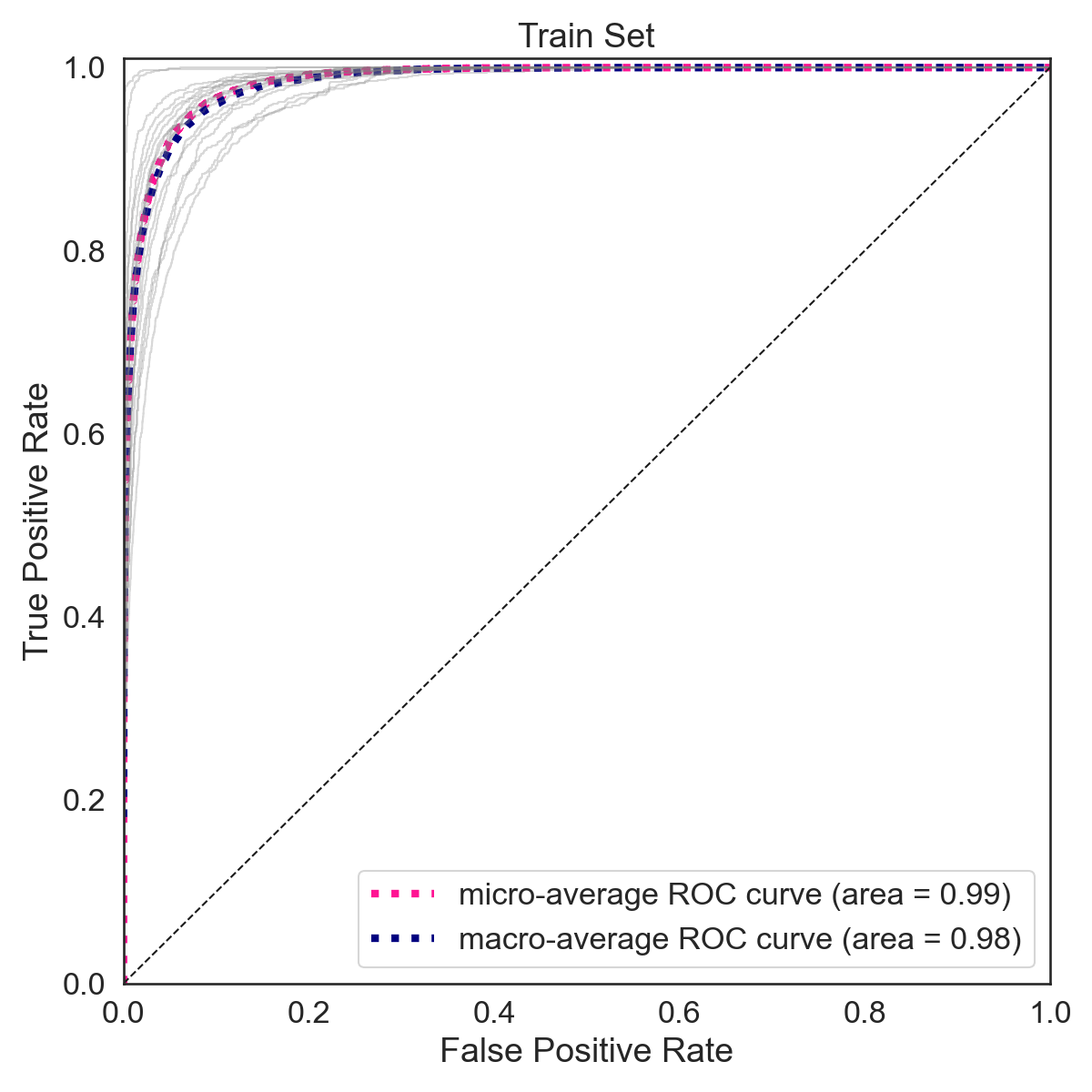 |  |
Predictions
 |  |
 | 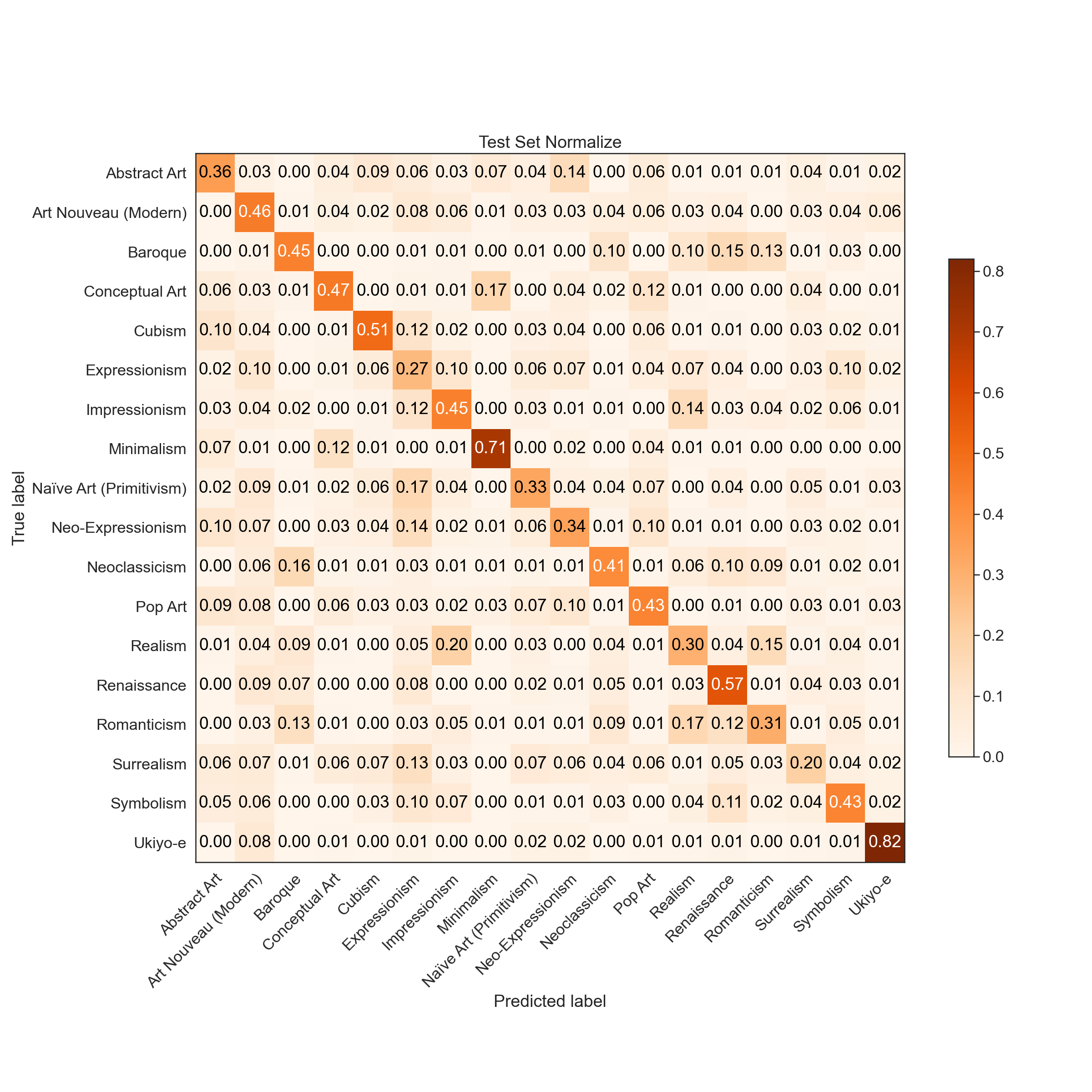 |
## load prediction reports
train_report = pd.read_csv("../models/1.d.1000/Train_Set_report.csv", index_col=0)[['precision', 'recall', 'f1-score']]
test_report = pd.read_csv("../models/1.d.1000/Test_Set_report.csv", index_col=0)[['precision', 'recall', 'f1-score']]

train_report = train_report.iloc[0:-3,:]
test_report = test_report.iloc[0:-3,:]

report = pd.merge(left=train_report, right=test_report, left_index=True, right_index=True, suffixes=('_train', '_test'))
## plot report
sns.set(font_scale = 1.5)
sns.set_style('whitegrid')

fig, ax = plt.subplots(figsize=(16,6))
report.plot(ax=ax, style=['--',':','-.','--',':','-.'], color=['b','r','g', 'orange', 'mediumpurple', 'crimson'])

ax.set_xticks(range(0,18))
ax.set_xticklabels(report.index, fontsize=15)
plt.xticks(rotation=45, ha = 'right')

ax.legend(loc='upper center', bbox_to_anchor=(1.1, 0.8),fancybox=True, shadow=True, ncol=1)
ax.set_title("Prediction Report")
ax.set_ylim(0, 1.)
ax.set_xlim(0, 17)
plt.tight_layout();
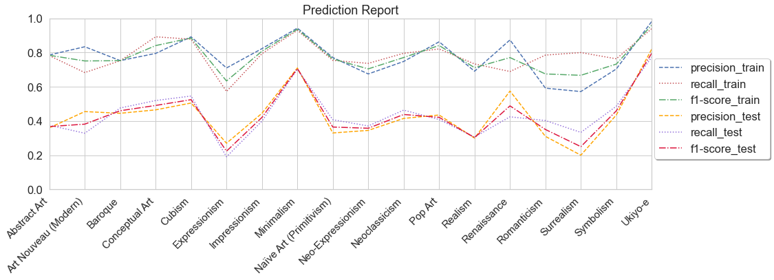
Transfer Learning - Third Generation
Training
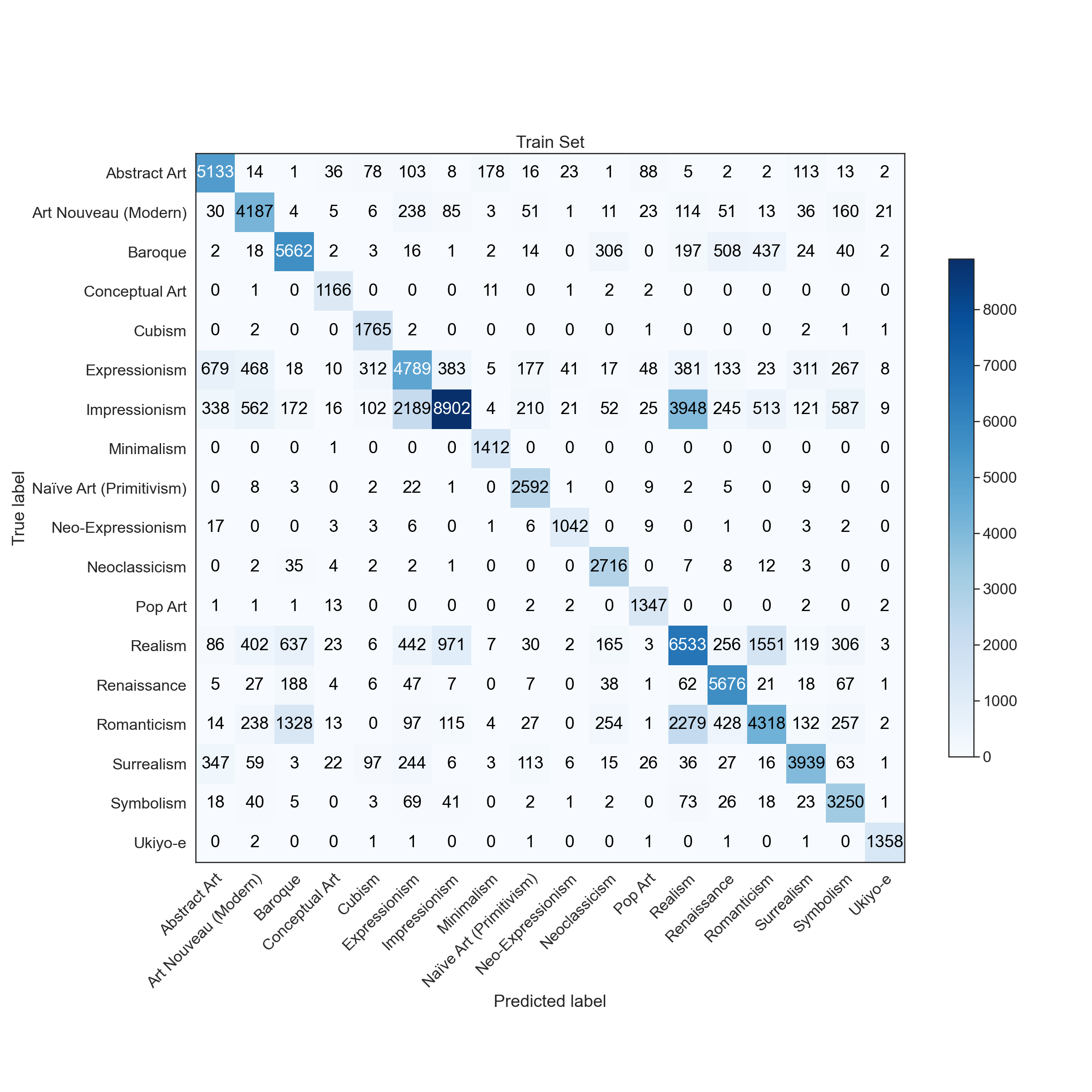
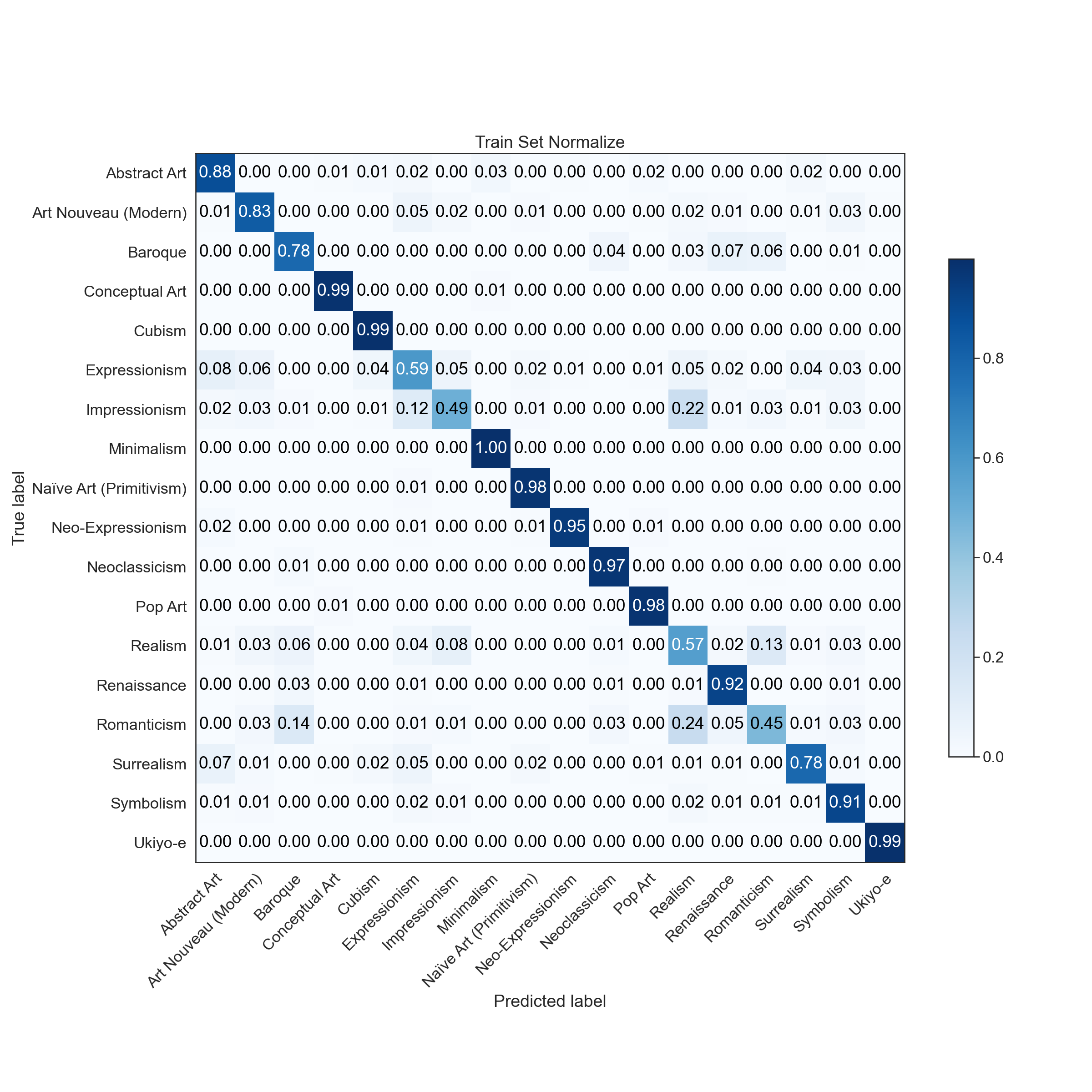
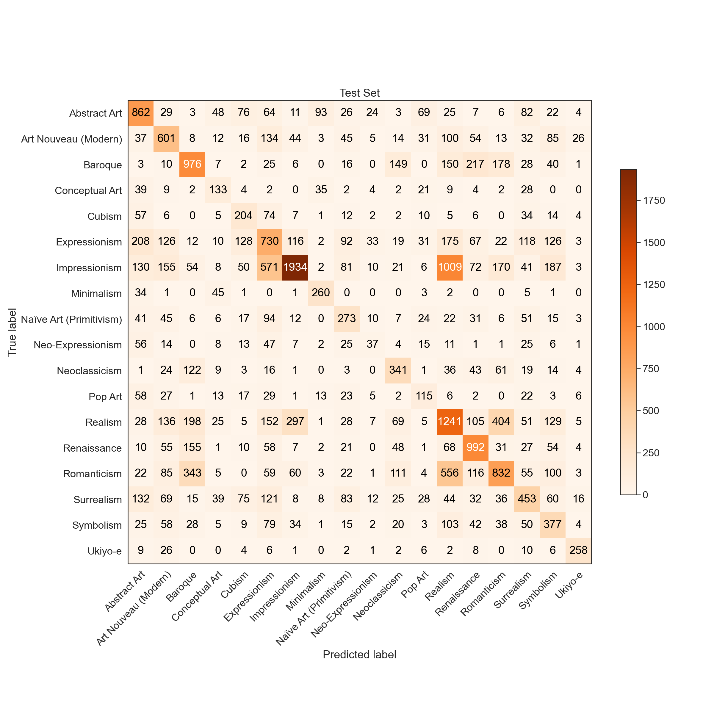
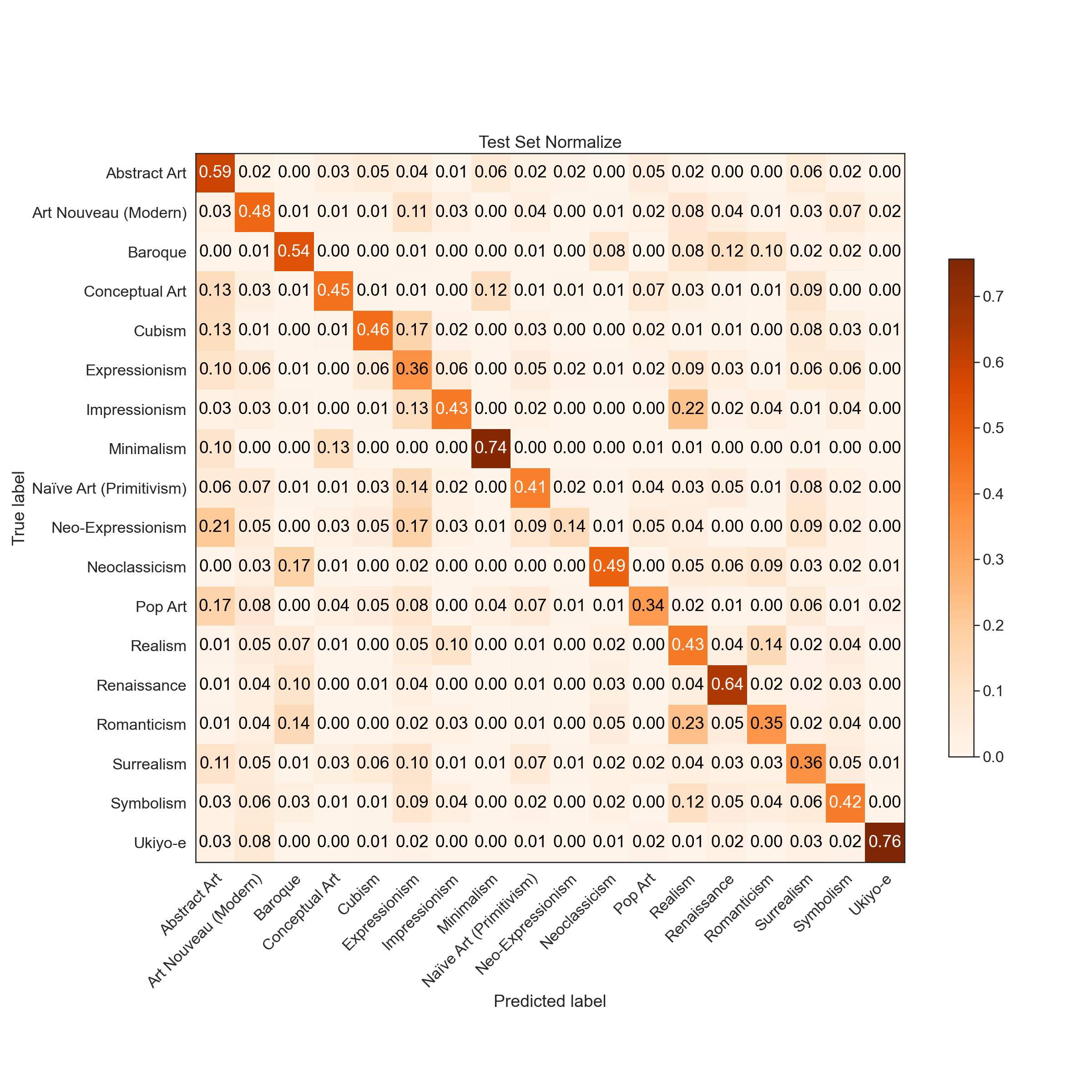
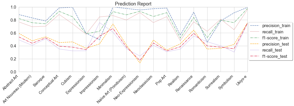
As shown below the training accuracy plateaus at 57% (benchmark accuracy is 5.6%) while the accuracy on the test set is 45%.
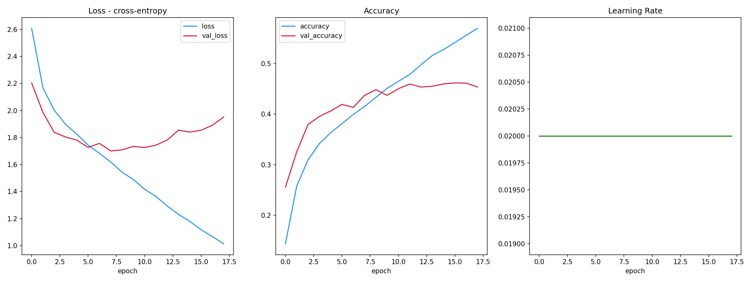
The F-1 score on the training set is 0.79 (macro average) and 0.71 (weighted average). The F-1 score on the training set is 0.45 (macro average) and 0.45 (weighted average).
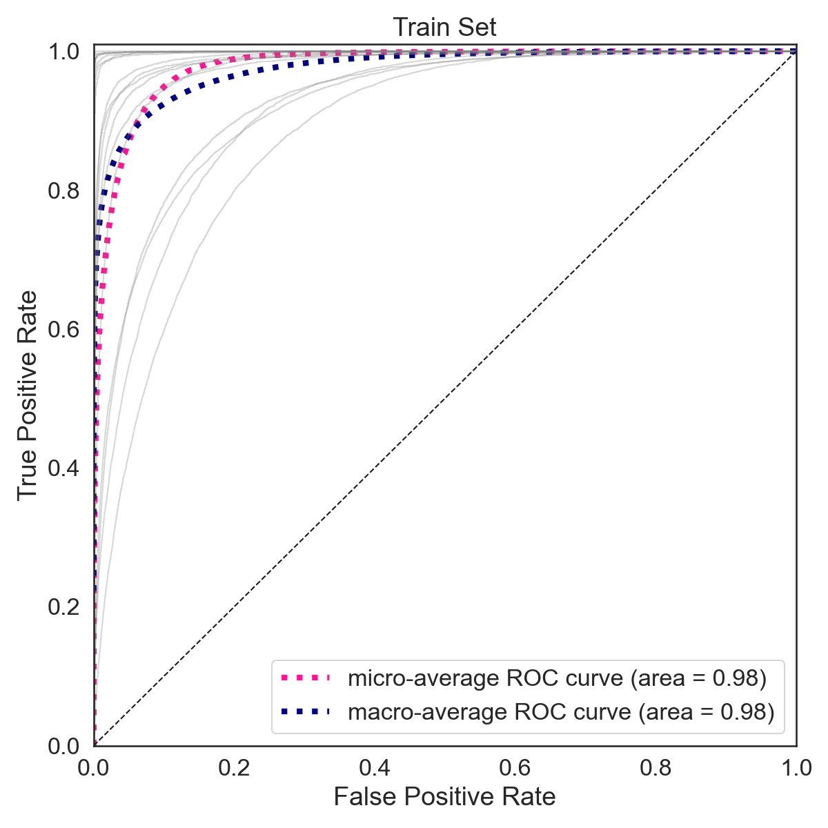 | 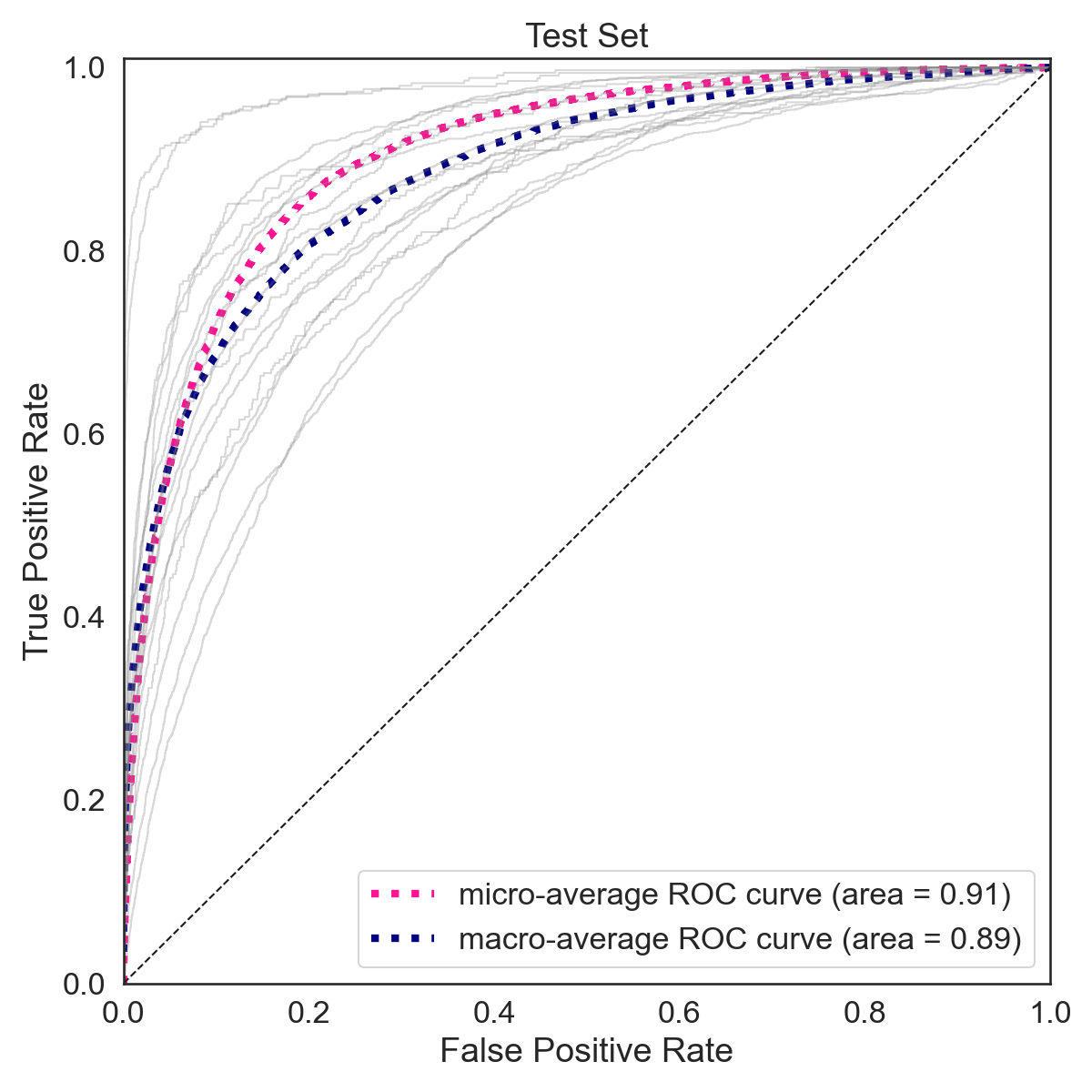 |
Predictions
 |  |
 |  |
## load prediction reports
train_report = pd.read_csv("../models/2_d/Train_Set_report.csv", index_col=0)[['precision', 'recall', 'f1-score']]
test_report = pd.read_csv("../models/2_d/Test_Set_report.csv", index_col=0)[['precision', 'recall', 'f1-score']]

train_report = train_report.iloc[0:-3,:]
test_report = test_report.iloc[0:-3,:]

report = pd.merge(left=train_report, right=test_report, left_index=True, right_index=True, suffixes=('_train', '_test'))
## plot report
sns.set(font_scale = 1.5)
sns.set_style('whitegrid')

fig, ax = plt.subplots(figsize=(16,6))
report.plot(ax=ax, style=['--',':','-.','--',':','-.'], color=['b','r','g', 'orange', 'mediumpurple', 'crimson'])

ax.set_xticks(range(0,18))
ax.set_xticklabels(report.index, fontsize=15)
plt.xticks(rotation=45, ha = 'right')

ax.legend(loc='upper center', bbox_to_anchor=(1.1, 0.8),fancybox=True, shadow=True, ncol=1)
ax.set_title("Prediction Report")
ax.set_ylim(0, 1.)
ax.set_xlim(0, 17)
plt.tight_layout();
References
[1] Wikiart, https://www.wikiart.org/
[2] Lucas Oliveira David, Wikiart Retrieval, GitHub