Titanic Disaster Study
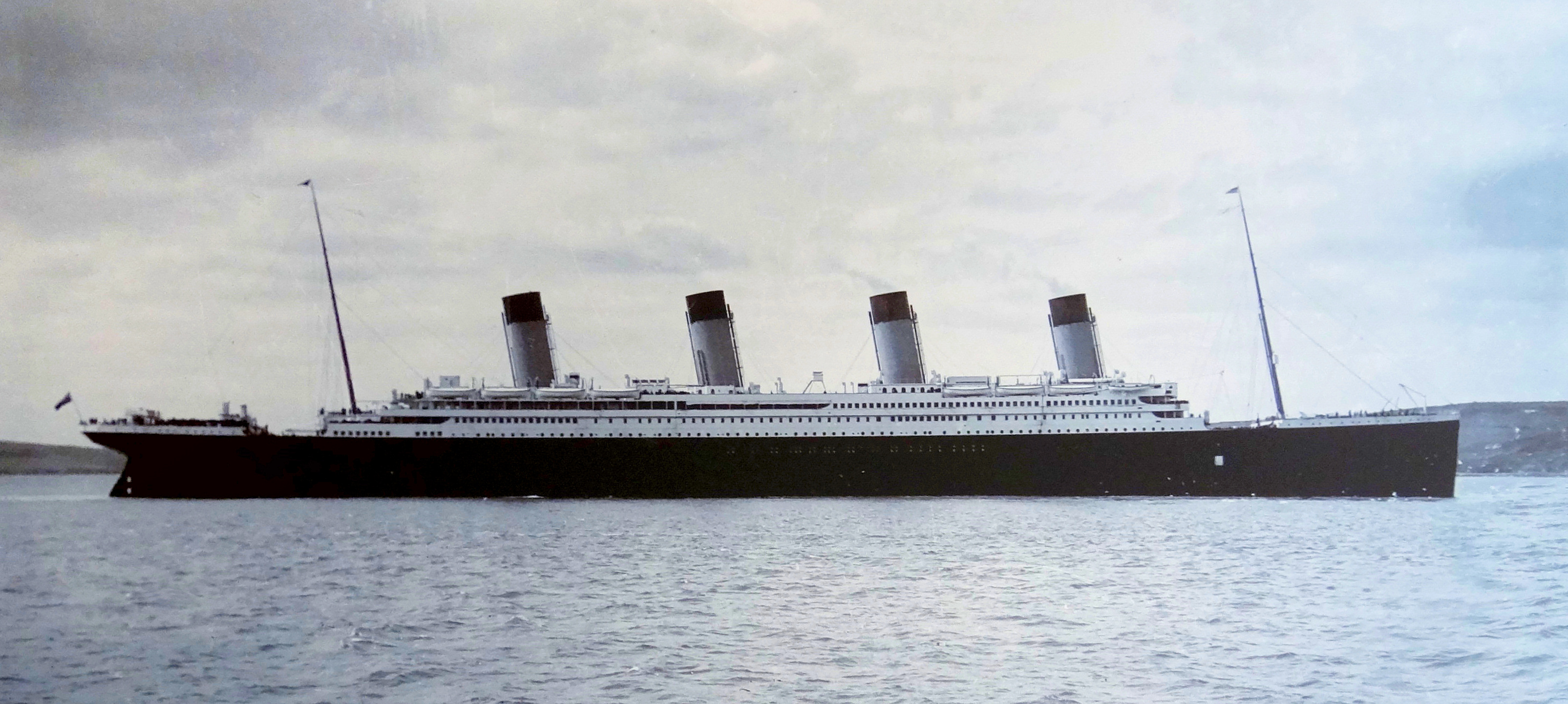
Table of Content
1. Introduction
2. Data Import
2.1 Import Libraries
2.2 Load specific tools
2.3 Data Import
2.4 Data Inspection
3. Data Exploration and Data Cleaning
3.1 Pivoting Features
3.2 Embarked Feature
3.3 Fare Feature
3.4 Cabin Feature
3.5 Age Feature
4. Data Visualization and Feature Exploration
4.1 Gender
4.2 Age
4.3 Pclass and Fare
4.4 SibSp & Parch
4.5 Embarked
5. Statistical Study
5.1 Main Features
5.2 Correlation Study
6. Feature Preparation
6.1 Passenger Title
6.2 Family Size
6.3 Tickets
6.4 Family Survival Rate
6.4 Fare Binning
6.4 Age Binning
6.4 Encoding
7. Model Preparation
8. Models
9. Best Models
10. Create Submission
1. Introduction
On April 15, 1912, the Titanic sunk after colliding with an iceberg, 1502 out of 2224 passengers and crew members died. The dataset containing passenger information has been made available. The purpose of this Notebook is to perform a comparison study of different models aimed at predicting survival rate. The data is obtained from Kaggle.
2. Data Import
2.1 Import Libraries
# Load libraries
import sys
print("Python version:\t\t{}".format(sys.version))
import pandas as pd
print("pandas version:\t\t{}".format(pd.__version__))
import matplotlib
print("matplotlib version:\t{}".format(matplotlib.__version__))
import numpy as np
print("numpy version:\t\t{}".format(np.__version__))
import scipy as sp
print("scipy version:\t\t{}".format(sp.__version__))
import sklearn
print("sklearn version:\t{}".format(sklearn.__version__))
Python version:		3.7.6 (default, Jan  8 2020, 20:23:39) [MSC v.1916 64 bit (AMD64)]
pandas version:		0.25.3
matplotlib version:	3.1.1
numpy version:		1.18.1
scipy version:		1.3.2
sklearn version:	0.22.1
2.2 Load specific tools
# Visualization
import matplotlib.pyplot as plt
import seaborn as sns
sns.set(style='whitegrid', context='notebook', palette='deep')
%matplotlib inline

# Models
from sklearn.model_selection import cross_val_score,GridSearchCV, StratifiedKFold, train_test_split
from sklearn.preprocessing import StandardScaler, LabelEncoder, OneHotEncoder

from sklearn.tree import DecisionTreeClassifier, DecisionTreeRegressor, ExtraTreeClassifier
from sklearn.naive_bayes import GaussianNB, BernoulliNB
from sklearn.tree import DecisionTreeClassifier
from sklearn.svm import SVC, NuSVC, LinearSVC
from sklearn.linear_model import LogisticRegression, PassiveAggressiveClassifier, RidgeClassifier, SGDClassifier, Perceptron
from sklearn.neighbors import KNeighborsClassifier
from sklearn.discriminant_analysis import LinearDiscriminantAnalysis, QuadraticDiscriminantAnalysis
from sklearn.neural_network import MLPClassifier
from sklearn.ensemble import AdaBoostClassifier, VotingClassifier, ExtraTreesClassifier, RandomForestClassifier, GradientBoostingClassifier, BaggingClassifier
from sklearn.gaussian_process import GaussianProcessClassifier
from sklearn.decomposition import PCA

from xgboost import XGBClassifier

# Tools
from sklearn.metrics import mean_squared_error, roc_auc_score, roc_curve, auc
from sklearn.metrics import accuracy_score,classification_report, precision_recall_curve, confusion_matrix
from sklearn.model_selection import cross_val_score, GridSearchCV, learning_curve

from collections import Counter
from tqdm import tqdm
import string


# Do not show warnings (added after Notebook was finalized)
import warnings
warnings.filterwarnings('ignore')
2.3 Data Import
We import both the training and test sets, we then combine them to compute statistics on the entire population of passengers.
# Import training and testing csv datasets
train = pd.read_csv('./Data/train.csv')
test = pd.read_csv('./Data/test.csv')
# Inspect data
train.head()
| PassengerId | Survived | Pclass | Name | Sex | Age | SibSp | Parch | Ticket | Fare | Cabin | Embarked | |
|---|---|---|---|---|---|---|---|---|---|---|---|---|
| 0 | 1 | 0 | 3 | Braund, Mr. Owen Harris | male | 22.0 | 1 | 0 | A/5 21171 | 7.2500 | NaN | S |
| 1 | 2 | 1 | 1 | Cumings, Mrs. John Bradley (Florence Briggs Th... | female | 38.0 | 1 | 0 | PC 17599 | 71.2833 | C85 | C |
| 2 | 3 | 1 | 3 | Heikkinen, Miss. Laina | female | 26.0 | 0 | 0 | STON/O2. 3101282 | 7.9250 | NaN | S |
| 3 | 4 | 1 | 1 | Futrelle, Mrs. Jacques Heath (Lily May Peel) | female | 35.0 | 1 | 0 | 113803 | 53.1000 | C123 | S |
| 4 | 5 | 0 | 3 | Allen, Mr. William Henry | male | 35.0 | 0 | 0 | 373450 | 8.0500 | NaN | S |
# Inspect data
test.head()
| PassengerId | Pclass | Name | Sex | Age | SibSp | Parch | Ticket | Fare | Cabin | Embarked | |
|---|---|---|---|---|---|---|---|---|---|---|---|
| 0 | 892 | 3 | Kelly, Mr. James | male | 34.5 | 0 | 0 | 330911 | 7.8292 | NaN | Q |
| 1 | 893 | 3 | Wilkes, Mrs. James (Ellen Needs) | female | 47.0 | 1 | 0 | 363272 | 7.0000 | NaN | S |
| 2 | 894 | 2 | Myles, Mr. Thomas Francis | male | 62.0 | 0 | 0 | 240276 | 9.6875 | NaN | Q |
| 3 | 895 | 3 | Wirz, Mr. Albert | male | 27.0 | 0 | 0 | 315154 | 8.6625 | NaN | S |
| 4 | 896 | 3 | Hirvonen, Mrs. Alexander (Helga E Lindqvist) | female | 22.0 | 1 | 1 | 3101298 | 12.2875 | NaN | S |
# tools functions: concat and divide
def concat_df(train, test):
    return pd.concat([train, test], sort=True).reset_index(drop=True)


def divide_df(full_df):
    return full_df.loc[:890], full_df.loc[891:].drop(['Survived'], axis=1)


df_all = concat_df(train, test)
# create a clone to test different transformations
df_exp = df_all.copy()
2.4 Data Inspection
The data is divided into two separate datasets:
- a training set containing a set of features and out target variable (whether or not a passenger survived)
- a test set containing only the set of features
Data Features
. Pclass: Categorical feature used to describe the passenger class (1=Upper, 2=Middle, 3=Lower).
. Name: String Containing a passenger name and title.
. Sex: Categorical variable describing the passenger’s gender.
. Age: Numerical feature standing for the passenger’s age.
. SibSp: Number of siblings/spouses aboard.
. Parch: Number of parents/children aboard.
. Ticket: Ticket number.
. Fare: Price of the ticket.
. Cabin: Cabin id.
. Embarked: Categorical feature, port of embarkation.
Target:
. Survived: Target feature (1=Survived, 0=Died)
3. Data Exploration and Data Cleaning
# Remove the Passengerid from the set as it does not need to be included in the models
passengerId = test.PassengerId

train = train.drop(['PassengerId'],axis=1)
test = test.drop(['PassengerId'],axis=1)
# list information for each feature (type, number of nun-null records)
train.info()
<class 'pandas.core.frame.DataFrame'>
RangeIndex: 891 entries, 0 to 890
Data columns (total 11 columns):
Survived    891 non-null int64
Pclass      891 non-null int64
Name        891 non-null object
Sex         891 non-null object
Age         714 non-null float64
SibSp       891 non-null int64
Parch       891 non-null int64
Ticket      891 non-null object
Fare        891 non-null float64
Cabin       204 non-null object
Embarked    889 non-null object
dtypes: float64(2), int64(4), object(5)
memory usage: 76.7+ KB
# list information for each feature (type, number of nun-null records)
test.info()
<class 'pandas.core.frame.DataFrame'>
RangeIndex: 418 entries, 0 to 417
Data columns (total 10 columns):
Pclass      418 non-null int64
Name        418 non-null object
Sex         418 non-null object
Age         332 non-null float64
SibSp       418 non-null int64
Parch       418 non-null int64
Ticket      418 non-null object
Fare        417 non-null float64
Cabin       91 non-null object
Embarked    418 non-null object
dtypes: float64(2), int64(3), object(5)
memory usage: 32.8+ KB
Comment:
Several of the features in the training set appear to be incomplete (Age, Cabin, and Embarked).
Several of the features in the test set appear to be incomplete (Age, Cabin, and Fare).
# compute percentage of missing values

# compute number of missing records
missing_total = train.isnull().sum().sort_values(ascending=False)

# convert to percentages
missing_percentage = missing_total/train.shape[0]*100

# display missing record %
print('Missing values in training set:')
pd.concat([missing_total,missing_percentage],keys=['Count','Percentage'],axis=1)
Missing values in training set:
| Count | Percentage | |
|---|---|---|
| Cabin | 687 | 77.104377 |
| Age | 177 | 19.865320 |
| Embarked | 2 | 0.224467 |
| Fare | 0 | 0.000000 |
| Ticket | 0 | 0.000000 |
| Parch | 0 | 0.000000 |
| SibSp | 0 | 0.000000 |
| Sex | 0 | 0.000000 |
| Name | 0 | 0.000000 |
| Pclass | 0 | 0.000000 |
| Survived | 0 | 0.000000 |
Comment:
Based on the above table, the following observations can be made:
- The cabin feature is mostly empty, this will be hard to use.
- The age feature contains a large number of missing values. This will require a smarter approach rather than just filling the null with a median.
- The embarked feature only has 2 missing values. We can come up with estimates for these two by taking a quick look at the data and using the most probable values as replacements.
# compute percentage of missing values

# compute number of missing records
missing_total = test.isnull().sum().sort_values(ascending=False)

# convert to percentages
missing_percentage = missing_total/train.shape[0]*100

# display missing record %
print('Missing values in test set:')
pd.concat([missing_total,missing_percentage],keys=['Count','Percentage'],axis=1)
Missing values in test set:
| Count | Percentage | |
|---|---|---|
| Cabin | 327 | 36.700337 |
| Age | 86 | 9.652076 |
| Fare | 1 | 0.112233 |
| Embarked | 0 | 0.000000 |
| Ticket | 0 | 0.000000 |
| Parch | 0 | 0.000000 |
| SibSp | 0 | 0.000000 |
| Sex | 0 | 0.000000 |
| Name | 0 | 0.000000 |
| Pclass | 0 | 0.000000 |
Comment:
Based on the above table, the following observations can be made:
- The cabin feature is also mostly empty, this will be hard to use.
- The age feature contains a large number of missing values. This will require a smarter approach rather than just filling the null with a median.
- The fare feature only has 1 missing values. We can come up with an estimate for this by taking a quick look at the data and using the most probable values as a replacement.
3.1 Pivoting features
Before diving in the data, it is interesting to get a quick overview of what is waiting for us. To do so, we can pivot several of the features with the target data and quickly identify which features seem important.
train[['Sex','Survived']].groupby(['Sex'],as_index=False).agg(['mean','count'])
| Survived | ||
|---|---|---|
| mean | count | |
| Sex | ||
| female | 0.742038 | 314 |
| male | 0.188908 | 577 |
train[['Pclass','Survived']].groupby(['Pclass'],as_index=False).agg(['mean','count'])
| Survived | ||
|---|---|---|
| mean | count | |
| Pclass | ||
| 1 | 0.629630 | 216 |
| 2 | 0.472826 | 184 |
| 3 | 0.242363 | 491 |
train[['SibSp','Survived']].groupby(['SibSp'],as_index=False).agg(['mean','count'])
| Survived | ||
|---|---|---|
| mean | count | |
| SibSp | ||
| 0 | 0.345395 | 608 |
| 1 | 0.535885 | 209 |
| 2 | 0.464286 | 28 |
| 3 | 0.250000 | 16 |
| 4 | 0.166667 | 18 |
| 5 | 0.000000 | 5 |
| 8 | 0.000000 | 7 |
train[['Parch','Survived']].groupby(['Parch'],as_index=False).agg(['mean','count'])
| Survived | ||
|---|---|---|
| mean | count | |
| Parch | ||
| 0 | 0.343658 | 678 |
| 1 | 0.550847 | 118 |
| 2 | 0.500000 | 80 |
| 3 | 0.600000 | 5 |
| 4 | 0.000000 | 4 |
| 5 | 0.200000 | 5 |
| 6 | 0.000000 | 1 |
In conclusion:
- Gender, Females have a higher change of survival over men (74% vs. 19%)
- Pclass, the survival rate is strongly correlated with the passenger class
- SibSp, Parch, smaller family tends to have a higher survival rate
3.2 Age
The age feature is likely important for the predictions, however, it contains a large number of missing values. We need to come up with a strategy to fill the missing values. Let’s start by computing the feature correlations to determine which feature is highly correlated to the age of the passengers.
# compute all correlations
df_all_corr = df_all.corr().abs()

# display correlations with age
print("Correlation with Age feature")
df_all_corr['Age'].sort_values(ascending=False)[1:]
Correlation with Age feature

Pclass         0.408106
SibSp          0.243699
Fare           0.178740
Parch          0.150917
Survived       0.077221
PassengerId    0.028814
Name: Age, dtype: float64
As listed above, the Class feature is fairly well correlated to the Age of the passenger. However, the listed correlation do not include the effects of binary features such as the gender. We can breakdown the correlations to include sub-divisions.
df_exp['Cat'] = df_exp['Sex'].astype(str) + df_exp['Pclass'].astype(str)
df_exp.groupby(['Cat']).median()['Age']
Cat
female1    36.0
female2    28.0
female3    22.0
male1      42.0
male2      29.5
male3      25.0
Name: Age, dtype: float64
From the above, we can see that for each class women seem to be younger than men. In addition, we can see that older passengers travels in higher class.
# fill missing age with groups Sex + PClass
df_all['Age'] = df_all.groupby(['Sex', 'Pclass'
                               ])['Age'].apply(lambda x: x.fillna(x.median()))

assert df_all['Age'].isnull().sum()==0
The age feature is now complete.
3.3 Embarked Feature
The embarked feature has missing values in the training set.
# Distribution of the data
train['Embarked'].value_counts(dropna=False)
S      644
C      168
Q       77
NaN      2
Name: Embarked, dtype: int64
We now inspect the rest of the records for these two missing values:
train[train['Embarked'].isnull()]
| Survived | Pclass | Name | Sex | Age | SibSp | Parch | Ticket | Fare | Cabin | Embarked | |
|---|---|---|---|---|---|---|---|---|---|---|---|
| 61 | 1 | 1 | Icard, Miss. Amelie | female | 38.0 | 0 | 0 | 113572 | 80.0 | B28 | NaN |
| 829 | 1 | 1 | Stone, Mrs. George Nelson (Martha Evelyn) | female | 62.0 | 0 | 0 | 113572 | 80.0 | B28 | NaN |
Let’s group the passenger with similar features:
- Female
- 1st Class
- Fare between 50 and 100
df_all[(df_all['Pclass'] == 1) & (df_all['Sex'] == 'female') &
       (df_all['Fare'] >= 50) & (df_all['Fare'] <= 100)].groupby(
           ['Embarked']).count()['Age']
Embarked
C    30
Q     2
S    35
Name: Age, dtype: int64
From the above, the most common embarked location is “S”. We will replace the missing values with this.
# Fill missing values
df_all['Embarked'].fillna('S',inplace=True)
3.4 Fare Feature
The test set has a missing value for the Fare feature.
# Display record corresponding to missing value
df_all[df_all.Fare.isnull()]
| Age | Cabin | Embarked | Fare | Name | Parch | PassengerId | Pclass | Sex | SibSp | Survived | Ticket | |
|---|---|---|---|---|---|---|---|---|---|---|---|---|
| 1043 | 60.5 | NaN | S | NaN | Storey, Mr. Thomas | 0 | 1044 | 3 | male | 0 | NaN | 3701 |
We will use the median Fare of the subset corresponding to Pclass=3, Embarked=’S’, Sex=’male’, Age>=21 (for adult).
# Extract median
subset_med = df_all[(df_all['Pclass'] == 3) & (df_all['SibSp'] == 0) &
                  (df_all['Parch'] == 0)]['Fare'].median()

# Replace missing value
df_all['Fare'] = df_all['Fare'].fillna(subset_med)
3.5 Cabin Feature
The cabin feature is missing for 77% of the training set and 78% of the test set. With such a high percentage, the feature can either be dropped or feature engineering can be used to understand how the cabin id is defined. We opt for the second option.
# Feature inspection
df_all['Cabin'].sort_values().head(5)
583     A10
1099    A11
475     A14
556     A16
1222    A18
Name: Cabin, dtype: object
By doing some research on the ship, the Cabin value contains the following information:
- One letter standing for the boat deck
- One number standing for the cabin number
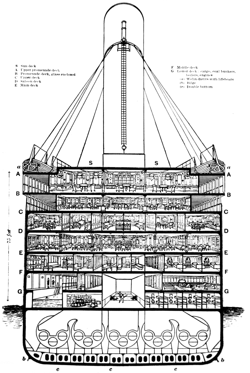
source: Wikipedia
# Extract deck name from cabine feature (replace with "M" (missing) if Cabin is null)
df_all['Deck'] = df_all['Cabin'].apply(lambda x: x[0] if pd.notnull(x) else "M")
df_plot = df_all.groupby(['Deck', 'Pclass']).size().reset_index().pivot(columns='Pclass', index='Deck', values=0)
df_plot.fillna(0)
| Pclass | 1 | 2 | 3 |
|---|---|---|---|
| Deck | |||
| A | 22.0 | 0.0 | 0.0 |
| B | 65.0 | 0.0 | 0.0 |
| C | 94.0 | 0.0 | 0.0 |
| D | 40.0 | 6.0 | 0.0 |
| E | 34.0 | 4.0 | 3.0 |
| F | 0.0 | 13.0 | 8.0 |
| G | 0.0 | 0.0 | 5.0 |
| M | 67.0 | 254.0 | 693.0 |
| T | 1.0 | 0.0 | 0.0 |
df_plot = df_plot.div(df_plot.sum(axis=1), axis=0)

fig, ax = plt.subplots(figsize=(16,6))
#ax = sns.countplot(x='Deck', data=df_all, hue='Pclass')
df_plot.plot(kind='bar', stacked=True, ax = ax)
ax.set_title('Class Distribution per Decks', fontsize=15)
ax.set_ylabel("Fraction of deck")
ax.legend()
ax.set_ylim(0,1);
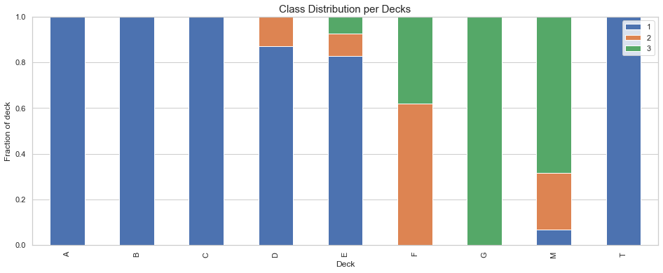
The following observations can be made from the above plot:
- Decks A, B, C are dedicated to the 1st class
- Decks D and E are mostly assigned to the 1st class
- Deck F is split for class 2 and 3
- Deck G is for the first class only
- Only one passenger is assigned to Deck T, this must be a mistake.
# move T Deck passenger to Deck A
idx = df_all[df_all['Deck'] == 'T'].index
df_all.loc[idx, 'Deck'] = 'A'
df_plot, _ = divide_df(df_all)
df_plot = df_plot.groupby(['Deck', 'Survived']).size().reset_index().pivot(
    columns='Survived', index='Deck').fillna(0).astype(int)
df_plot = df_plot.div(df_plot.sum(axis=1), axis=0)

fig, ax = plt.subplots(figsize=(16,6))
#ax = sns.countplot(x='Deck', data=df_all, hue='Pclass')
df_plot.plot(kind='bar', stacked=True, ax = ax, color=['r', 'b'])
ax.set_title('Survival Rate per Decks', fontsize=15)
ax.set_ylabel("Survival Rate")
ax.legend()
ax.set_ylim(0,1);
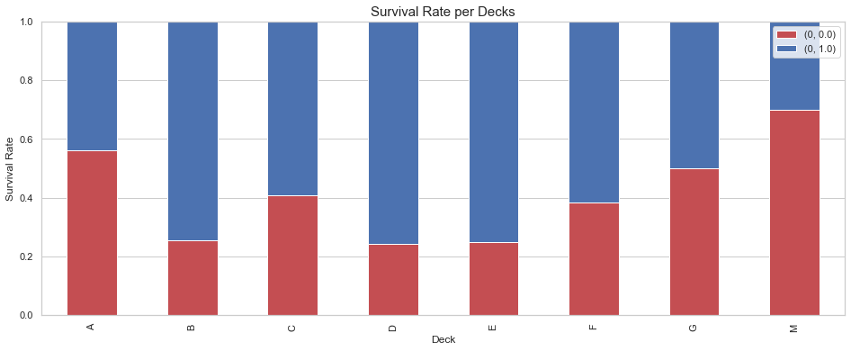
We can now group decks based on the survival rate and the class distribution.
We group:
- A, B, C since they exclusively contain 1st class passengers.
- D and E as they mostly contain 1st class passengers.
- F and G as they contain 2nd and 3rd class while having as similar survival rate.
df_all['Deck'] = df_all['Deck'].replace(['A', 'B', 'C'], 'ABC')
df_all['Deck'] = df_all['Deck'].replace(['D', 'E'], 'DE')
df_all['Deck'] = df_all['Deck'].replace(['F', 'G'], 'FG')
# drop cabin
df_all = df_all.drop(['Cabin'], axis=1)
At this point, we have filled all the missing values.
train, test = divide_df(df_all)
4. Data Visualization and Feature Exploration
Before we implement the full model, it is important to inspect the data and answers a few basic questions. This will help understanding how the data is distributed but also will provide useful input used in our models.
Based on the famous rule “Women and children first”, we expect the gender and age to be strongly correlated with the survival rate.
Questions:
- Gender: Is the survival rate higher for females?
- Age: Is the survival rate higher for young passengers?
- Pclass & Fare: Is the survival rate higher amongst wealthy passengers?
- SibSp & Parch: Is the survival rate for family is higher than the one for single passenger?
4.1 Gender
# Plot the box plot
pal = {'female':"salmon",'male':"skyblue"}
plt.subplots(figsize = (6,6))
ax = sns.barplot(x = "Sex", y = "Survived", data=train, palette = pal)
plt.title("Impact of gender on the survival rate",fontsize=15)
plt.ylabel("Survival rate",fontsize=15)
plt.xlabel("Sex",fontsize=15);
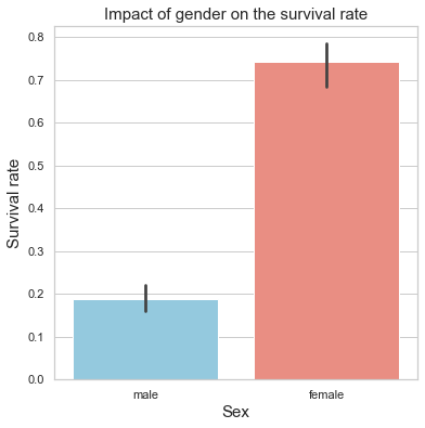
print("Male mean survival rate = \t {:.2f}%".format(train[train['Sex'] =='male']['Survived'].mean()*100))
print("Female mean survival rate = \t {:.2f}%".format(train[train['Sex'] != 'male']['Survived'].mean()*100))
Male mean survival rate = 	 18.89%
Female mean survival rate = 	 74.20%
Comment
Based on the boxplot, the gender appears to be a critical feature when it comes to determining the faith of a passenger. Indeed, females seem to have on average a much higher survival rate.
4.2 Age
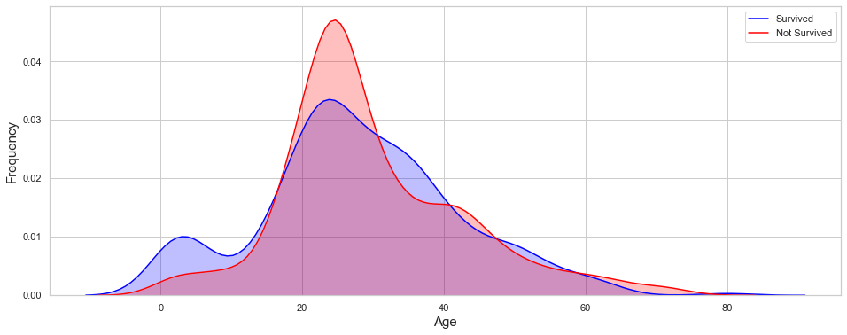
# Plot kernel density plot
fig, ax = plt.subplots(figsize=(16,6))
ax = sns.kdeplot(train.loc[(train['Survived']==1),'Age'],shade=True,color='blue',label='Survived');
ax = sns.kdeplot(train.loc[(train['Survived']==0),'Age'],shade=True,color='red',label='Not Survived')
ax.set_ylabel('Frequency',fontsize=15)
ax.set_xlabel('Age',fontsize=15);
print("Toddler survival rate = \t{:.2f}%".format(train[train['Age'] <= 2]['Survived'].mean()*100,2))
print("Children survival rate = \t{:.2f}%".format(train[(train['Age'] > 2) & (train['Age'] <= 12)]['Survived'].mean()*100,2))
print("Teenager survival rate = \t{:.2f}%".format(train[(train['Age'] > 12) & (train['Age'] <= 18)]['Survived'].mean()*100,2))
print("Young Adult survival rate = \t{:.2f}%".format(train[(train['Age'] > 18) & (train['Age'] <= 34)]['Survived'].mean()*100,2))
print("Adult survival rate = \t\t{:.2f}%".format(train[(train['Age'] > 34) & (train['Age'] <= 50)]['Survived'].mean()*100,2))
print("pre-senior survival rate = \t{:.2f}%".format(train[(train['Age'] > 50) & (train['Age'] <= 70)]['Survived'].mean()*100,2))
print("senior survival rate = \t\t{:.2f}%".format(train[train['Age'] > 70]['Survived'].mean()*100,2))
Toddler survival rate = 	62.50%
Children survival rate = 	55.56%
Teenager survival rate = 	42.86%
Young Adult survival rate = 	33.74%
Adult survival rate = 		42.57%
pre-senior survival rate = 	35.59%
senior survival rate = 		20.00%
Comment
Based on the distribution plot, the age also appears to be a critical feature. Young children have a much higher survival rate on average than the rest of the passenger. The survival rate tends to decrease with the age.
4.3 Pclass and Fare
# Plot the survival rate per class
pal = {1:"gold",2:"silver",3:'sandybrown'}
plt.subplots(figsize = (6,6))
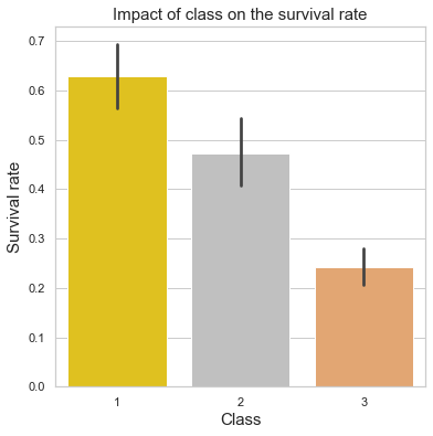
ax = sns.barplot(x = "Pclass", y = "Survived", data=train, palette = pal)
plt.title("Impact of class on the survival rate",fontsize=15)
plt.ylabel("Survival rate",fontsize=15)
plt.xlabel("Class",fontsize=15);
print("Upper class survival rate =\t{:.2f}%".format(train[train['Pclass'] == 1]['Survived'].mean()*100))
print("Middle class survival rate =\t{:.2f}%".format(train[train['Pclass'] == 2]['Survived'].mean()*100))
print("Lower class survival rate =\t{:.2f}%".format(train[train['Pclass'] == 3]['Survived'].mean()*100))
Upper class survival rate =	62.96%
Middle class survival rate =	47.28%
Lower class survival rate =	24.24%
Comment
The above plot confirms our assumption: upper class passengers had a much higher survival rate.
Before we look at the impact of the fare on the survival rate, we need to verify how the class is correlated to the fare.
# Plot the survival rate per class
pal = {1:"gold",2:"silver",3:'sandybrown'}
plt.subplots(figsize = (6,6))
ax = sns.barplot(x = "Pclass", y = "Fare", data=train, palette = pal)
plt.title("Impact of the passenger class on the fare",fontsize=15)
plt.ylabel("Fare",fontsize=15)
plt.xlabel("Pclass",fontsize=15);
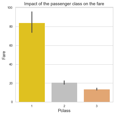
print('Median fare:')
print("1st class =\t$${:.2f}".format(train[train['Pclass'] == 1]['Fare'].median()))
print("2nd class =\t$${:.2f}".format(train[train['Pclass'] == 2]['Fare'].median()))
print("3nd class =\t$${:.2f}".format(train[train['Pclass'] == 3]['Fare'].median()))
Median fare:
1st class =	$$60.29
2nd class =	$$14.25
3nd class =	$$8.05
# Box plot
fig, ax = plt.subplots(figsize=(16,6))
sns.boxplot(x = 'Pclass', y = 'Fare', hue = 'Survived', data = train, ax = ax)
ax.set_title('Pclass vs Fare Survival Comparison',fontsize=15)
ax.set_ylim(0, 300);
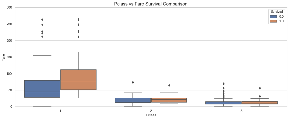
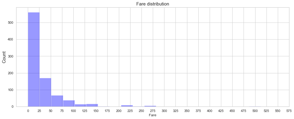
fig = plt.figure(figsize=(16,6),)
ax=sns.distplot(train['Fare'] , color='blue',kde=False,bins=20)
ax.set_ylabel("Count",fontsize=15)
ax.set_title('Fare distribution',fontsize=15)
ax.set_xticks(range(0,600,25));
# Kernel Density Plot
fig = plt.figure(figsize=(16,6))
ax=sns.distplot(train.loc[(train['Survived'] == 0),'Fare'] , color='red',label='Not Survived',kde=False,bins=21)
ax=sns.distplot(train.loc[(train['Survived'] == 1),'Fare'] , color='blue', label='Survived',kde=False,bins=41)
ax.legend(['Not Survived','Survived'])
plt.xlabel("Fare",fontsize=15)
plt.ylabel("Frequency of Passenger Survived",fontsize=15)
plt.title('Fare Distribution Survived vs Non Survived',fontsize=15);
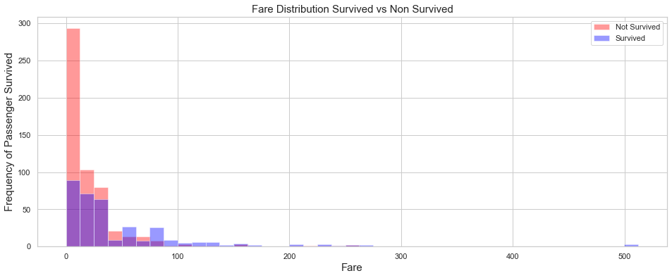
Comment
As expected. the survival rate increases with the fare price. Based on the above plot, it appears that the survival rate is larger than 50% for fares higher that $$150.
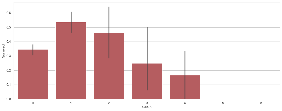
4.4 SibSp & Parch
train[['SibSp','Survived']].groupby(['SibSp'],as_index=False).mean().sort_values(by='Survived',ascending =False)
| SibSp | Survived | |
|---|---|---|
| 1 | 1 | 0.535885 |
| 2 | 2 | 0.464286 |
| 0 | 0 | 0.345395 |
| 3 | 3 | 0.250000 |
| 4 | 4 | 0.166667 |
| 5 | 5 | 0.000000 |
| 6 | 8 | 0.000000 |
fig, ax = plt.subplots(figsize=(16,6))
sns.barplot(x="SibSp", y="Survived",color='r',data=train);
train[['Parch','Survived']].groupby(['Parch'],as_index=False).mean().sort_values(by='Survived',ascending =False)
| Parch | Survived | |
|---|---|---|
| 3 | 3 | 0.600000 |
| 1 | 1 | 0.550847 |
| 2 | 2 | 0.500000 |
| 0 | 0 | 0.343658 |
| 5 | 5 | 0.200000 |
| 4 | 4 | 0.000000 |
| 6 | 6 | 0.000000 |
fig, ax = plt.subplots(figsize=(16,6))
sns.barplot(x="Parch", y="Survived",color='b', data=train);
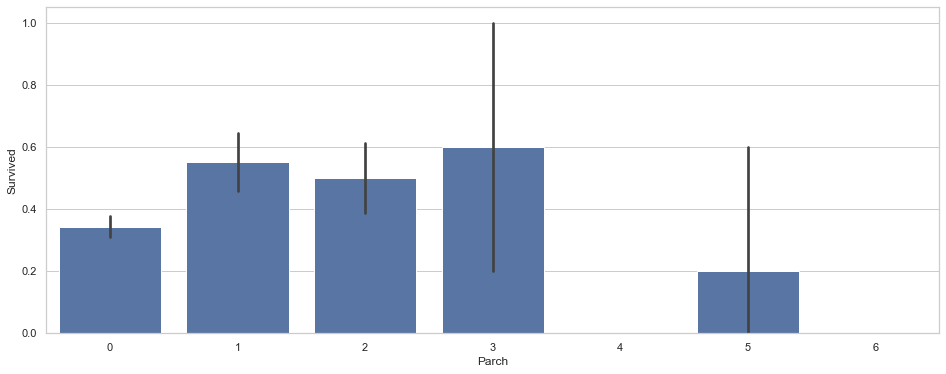
Comment
Passenger traveling with large family decreased the survival rate.
4.5 Embarked
train[['Embarked','Survived']].groupby(['Embarked'],as_index=False).mean().sort_values(by='Survived',ascending =False)
| Embarked | Survived | |
|---|---|---|
| 0 | C | 0.553571 |
| 1 | Q | 0.389610 |
| 2 | S | 0.339009 |
5. Statistical Study
In this section, we will inspect the data and quantify the observations that result from the data visualization.
5.1 Main Features
# Turning the Sex feature into a boolean classifier
train['Sex'] = train['Sex'].apply(lambda x: 0 if x == "female" else 1)
test['Sex'] = test['Sex'].apply(lambda x: 0 if x == "female" else 1)
train.describe()
| Age | Fare | Parch | PassengerId | Pclass | Sex | SibSp | Survived | |
|---|---|---|---|---|---|---|---|---|
| count | 891.000000 | 891.000000 | 891.000000 | 891.000000 | 891.000000 | 891.000000 | 891.000000 | 891.000000 |
| mean | 29.188182 | 32.204208 | 0.381594 | 446.000000 | 2.308642 | 0.647587 | 0.523008 | 0.383838 |
| std | 13.337887 | 49.693429 | 0.806057 | 257.353842 | 0.836071 | 0.477990 | 1.102743 | 0.486592 |
| min | 0.420000 | 0.000000 | 0.000000 | 1.000000 | 1.000000 | 0.000000 | 0.000000 | 0.000000 |
| 25% | 22.000000 | 7.910400 | 0.000000 | 223.500000 | 2.000000 | 0.000000 | 0.000000 | 0.000000 |
| 50% | 26.000000 | 14.454200 | 0.000000 | 446.000000 | 3.000000 | 1.000000 | 0.000000 | 0.000000 |
| 75% | 36.000000 | 31.000000 | 0.000000 | 668.500000 | 3.000000 | 1.000000 | 1.000000 | 1.000000 |
| max | 80.000000 | 512.329200 | 6.000000 | 891.000000 | 3.000000 | 1.000000 | 8.000000 | 1.000000 |
Comment
From the statistical data above, it appears that only 38% of the passengers survived.
train[['Sex', 'Survived']].groupby("Sex").mean()
| Survived | |
|---|---|
| Sex | |
| 0 | 0.742038 |
| 1 | 0.188908 |
train[['Pclass', 'Survived']].groupby("Pclass").mean()
| Survived | |
|---|---|
| Pclass | |
| 1 | 0.629630 |
| 2 | 0.472826 |
| 3 | 0.242363 |
5.2 Correlation Study
# Feature correlation
train.corr()['Survived'].sort_values()
Sex           -0.543351
Pclass        -0.338481
Age           -0.058635
SibSp         -0.035322
PassengerId   -0.005007
Parch          0.081629
Fare           0.257307
Survived       1.000000
Name: Survived, dtype: float64
# Compute the correlation matrix
corr = train.corr()

# Generate a mask for the upper triangle
mask = np.zeros_like(corr, dtype=np.bool)
mask[np.triu_indices_from(mask)] = True

# Set up the matplotlib figure
f, ax = plt.subplots(figsize=(10, 12))

# Generate a custom diverging colormap
cmap = sns.diverging_palette(220, 10, as_cmap=True)

# Draw the heatmap with the mask and correct aspect ratio
ax = sns.heatmap(corr, mask=mask, cmap=cmap, vmax=1.0,vmin=-1.0, center=0,annot=True,
            square=True, linewidths=.5, cbar_kws={"shrink": .5})

ylabels = [x.get_text() for x in ax.get_yticklabels()]
plt.yticks(np.arange(len(ylabels))+0.5,ylabels, rotation=0, fontsize="10", va="center")
ax.set_ylim(8,0.5);
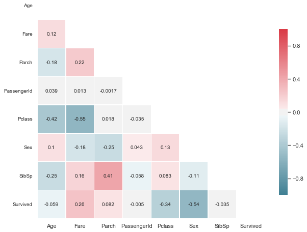
Comment
Strong positive correlations:
- Parch and SibSp (0.41)
- Fare and Survived (0.26)
- Parch and Fare (0.22)
Strong negative correlation
- Fare and Pclass (-0.42)
- Pclass and Age (-0.42)
- Pclass and Survived (-0.34)
6. Feature Preparation
Based on the knowledge gathered, we can now create new features that will help improve the model accuracy.
6.1 Passenger Title
Upon inspection of the Name feature, it appear that a title is assigned to each passenger. We extract this feature and store it in the dataset.
# extrace new feature using regular expression
df_all['Title'] = df_all['Name'].str.extract(r' ([A-Za-z]+)\.',expand=False)
df_all['Is_Married'] = 0
df_all['Is_Married'].loc[df_all['Title']=='Mrs'] = 1
fig, ax = plt.subplots(figsize=(16,6))
sns.barplot(x=df_all['Title'].value_counts().index, y=df_all['Title'].value_counts().values, ax=ax)
ax.set_title("Title Distribution");
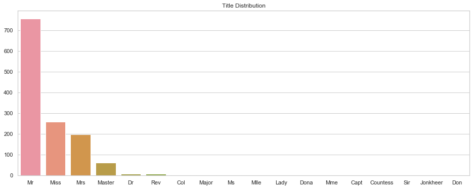
There are four principle titles. The rest consists of mostly single values. We can see if the survival rate varies between titles.
df_plot, _ = divide_df(df_all)
df_plot = df_plot.groupby(['Title', 'Survived']).size().reset_index().pivot(columns='Survived', index='Title').fillna(0).astype(int)
df_plot = df_plot.div(df_plot.sum(axis=1), axis=0)

fig, ax = plt.subplots(figsize=(16,6))
#ax = sns.countplot(x='Deck', data=df_all, hue='Pclass')
df_plot.plot(kind='bar', stacked=True, ax = ax, color=['r', 'b'])
ax.set_title('Survival Rate per Decks', fontsize=15)
ax.set_ylabel("Survival Rate")
ax.legend(['Not Survived', 'Survived'], loc="upper right")
ax.set_ylim(0,1);
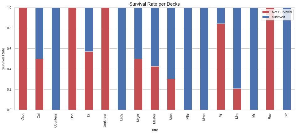
Based on the results shown above, it appears that different title are used to describe the same status. For instance Miss, Mlle, and Ms are used to describe Miss. We standardize the titles using a custom function.
df_all['Title'] = df_all['Title'].replace(
    ['Miss', 'Mrs', 'Ms', 'Mlle', 'Lady', 'Mme', 'Countess', 'Dona'],'Miss/Mrs/Ms')
df_all['Title'] = df_all['Title'].replace(
    ['Dr', 'Col', 'Major', 'Jonkheer', 'Capt', 'Sir', 'Don', 'Rev'], 'Rare')
df_plot, _ = divide_df(df_all)
df_plot = df_plot.groupby(['Title', 'Survived']).size().reset_index().pivot(
    columns='Survived', index='Title').fillna(0).astype(int)
df_plot = df_plot.div(df_plot.sum(axis=1), axis=0)

fig, axes = plt.subplots(1, 2, figsize=(16,6))
df_plot.plot(kind='bar', stacked=True, ax = axes[0], color=['r', 'b'])
axes[0].set_title('Survival Rate per Decks', fontsize=15)
axes[0].set_ylabel("Survival Rate")
axes[0].legend(['Not Survived', 'Survived'], loc="upper right")
axes[0].set_ylim(0,1)

sns.barplot(x=df_all['Title'].value_counts().index, y=df_all['Title'].value_counts().values, ax=axes[1])
axes[1].set_title("Title Distribution");
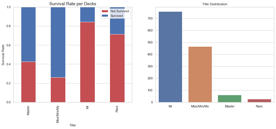
As displayed above the passenger title influences the survival rate.
6.2 Family Size
We can create a new feature used to calculate the size of the family:
df_all['Family_Size'] = df_all['Parch'] + df_all['SibSp'] + 1
fig, axes = plt.subplots(1, 2, figsize=(16, 6))

sns.barplot(x=df_all['Family_Size'].value_counts().index,
            y=df_all['Family_Size'].value_counts(),
            ax=axes[0])
axes[0].set_title("Family Size Distribution", fontsize=15)
sns.countplot(x='Family_Size',
              hue='Survived',
              data=df_all,
              ax=axes[1],
              palette=sns.diverging_palette(10, 255, sep=80, n=2))
axes[1].legend(['Not Survived', 'Survived'], loc='upper right')
axes[1].set_title("Survival Rate based on Family Size", fontsize=15)
Text(0.5, 1.0, 'Survival Rate based on Family Size')
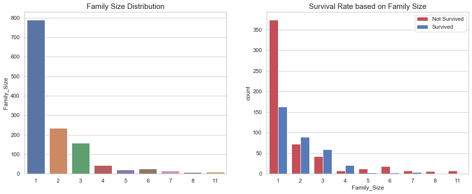
As shown above, single individual tend to die more than families of 2, 3, and 4 individuals. However, larger families suffer more casualties.
# group family sizes
family_map = {
    1: 'Alone',
    2: 'Small',
    3: 'Small',
    4: 'Small',
    5: 'Medium',
    6: 'Medium',
    7: 'Large',
    8: 'Large',
    11: 'Large'
}

df_all['Family_Size_Grp'] = df_all['Family_Size'].map(family_map)
fig, axes = plt.subplots(1, 2, figsize=(16, 6))

sns.barplot(x=df_all['Family_Size_Grp'].value_counts().index,
            y=df_all['Family_Size_Grp'].value_counts(),
            ax=axes[0])
axes[0].set_title("Family Size Distribution", fontsize=15)
sns.countplot(x='Family_Size_Grp', hue='Survived', data=df_all, ax=axes[1], palette=sns.diverging_palette(10, 255, sep=80, n=2))
axes[1].legend(['Not Survived', 'Survived'], loc='upper right')
axes[1].set_title("Survival Rate based on Family Size", fontsize=15);
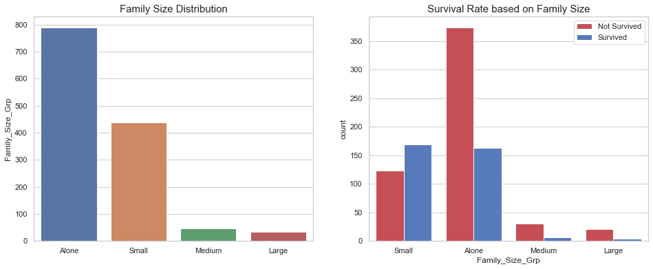
Based on our observations, we have grouped the family sizes into four groups. However, this new feature does not account for people not related but traveling in groups.
6.3 Tickets
We have not used the ticket id yet, If we simply try to group them, maybe we can obtain something interesting.
df_all.groupby('Ticket').size().sort_values(ascending=False)
Ticket
CA. 2343        11
1601             8
CA 2144          8
S.O.C. 14879     7
PC 17608         7
                ..
349248           1
349247           1
349246           1
349245           1
345769           1
Length: 929, dtype: int64
Indeed, the ticket seemed to have been assigned to groups of people rather than being unique. Let’s replace the actual tickets id as they do not see to contain a pattern.
df_all['Ticket_Frequency'] = df_all.groupby('Ticket')['Ticket'].transform('count')
fig, axes = plt.subplots(1, 2, figsize=(16, 6))

sns.barplot(x=df_all['Ticket_Frequency'].value_counts().index,
            y=df_all['Ticket_Frequency'].value_counts(),
            ax=axes[0])
axes[0].set_title("Ticket Frequency Distribution", fontsize=15)
sns.countplot(x='Ticket_Frequency', hue='Survived', data=df_all, ax=axes[1], palette=sns.diverging_palette(10, 255, sep=80, n=2))
axes[1].legend(['Not Survived', 'Survived'], loc='upper right')
axes[1].set_title("Survival Rate based on  Ticket Frequency", fontsize=15);
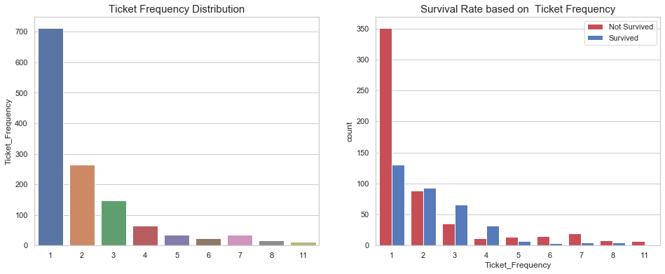
Similar to the family size, single individual tend to die more than families of 2, 3, and 4 individuals. However, larger families suffer more casualties.
6.4 Family Survival Rates
Based on the passenger last names, we can construct statistics related to individual families.
df_all['Last_Name'] = df_all['Name'].str.extract(r'^([a-zA-Z\s\-\']+)\,*')
If we want to compute the survival rate per family, we need to restrain our dataset to the training set since the test set does not contained the target feature.
df_train, df_test = divide_df(df_all)
In order to generate our new features, we need to perform the following steps:
- Find last names present in both the training and test sets.
- Compute median survival rate for each ticket and family.
- Save survival rates for families present in both test with more that one member. Same for tickets.
- Combine ticket and family survival rates
# 1. families and tickets occuring in both sets
non_unique_families = df_train.loc[df_train['Last_Name'].isin(df_test['Last_Name'].unique()), 'Last_Name']
non_unique_tickets = df_train.loc[df_train['Ticket'].isin(df_test['Ticket'].unique()), 'Ticket']
# 2. compute median survival rate and size for each ticket and family
df_family = df_train.groupby('Last_Name').median()[['Survived', 'Family_Size']]
df_ticket = df_train.groupby('Ticket').median()[['Survived', 'Ticket_Frequency']]
# 3. filter families with more that one member and present in both the train and test sets
df_family = df_family.loc[(df_family.index.isin(non_unique_families)) & (df_family['Family_Size']>1)][['Survived']]
df_ticket = df_ticket.loc[(df_ticket.index.isin(non_unique_tickets)) & (df_ticket['Ticket_Frequency']>1)][['Survived']]
# 3. compute mean survival rate
mean_survival_rate = np.mean(df_train['Survived'])
# 3.
# assign family survival rate to each passenger, same for tickets
df_train = df_train.merge(right=df_family, how='left', left_on='Last_Name',right_index=True, suffixes=('', '_y'))
df_train = df_train.rename(columns={"Survived_y": "Family_Survival"})
df_train = df_train.merge(right=df_ticket, how='left', left_on='Ticket',right_index=True, suffixes=('', '_y'))
df_train = df_train.rename(columns={"Survived_y": "Ticket_Survival"})

df_test = df_test.merge(right=df_family, how='left', left_on='Last_Name', right_index=True, suffixes=('', '_y'))
df_test = df_test.rename(columns={"Survived": "Family_Survival"})
df_test = df_test.merge(right=df_ticket, how='left', left_on='Ticket', right_index=True, suffixes=('', '_y'))
df_test = df_test.rename(columns={"Survived": "Ticket_Survival"})

# new feature to determine if a family has a family-based survival rate, same for tickets
df_train['Has_Family_Survival'] = (~df_train['Family_Survival'].isnull()).astype(int)
df_test['Has_Family_Survival'] = (~df_test['Family_Survival'].isnull()).astype(int)
df_train['Has_Ticket_Survival'] = (~df_train['Ticket_Survival'].isnull()).astype(int)
df_test['Has_Ticket_Survival'] = (~df_test['Ticket_Survival'].isnull()).astype(int)

# fill null with mean survival rate, same for tickets
df_train['Family_Survival'] = df_train['Family_Survival'].fillna(mean_survival_rate)
df_test['Family_Survival'] = df_test['Family_Survival'].fillna(mean_survival_rate)
df_train['Ticket_Survival'] = df_train['Ticket_Survival'].fillna(mean_survival_rate)
df_test['Ticket_Survival'] = df_test['Ticket_Survival'].fillna(mean_survival_rate)
# 4. Combine survival rates (Family and Ticket)
for df in [df_train, df_test]:
    df['Survival_Rate'] = (df['Ticket_Survival'] + df['Family_Survival']) / 2
    df['Has_Survival'] = (df['Has_Ticket_Survival'] + df['Has_Family_Survival']) / 2
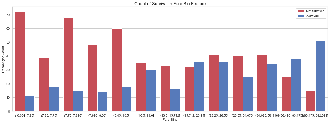
6.5 Fare Binning
In order to improve our predictions on unseen data, it is common to bin continuous features. Therefore, we bin the fare using quantiles. We select a number of bins with the intent to create bins as pure as possible.
df_all = concat_df(df_train, df_test)
df_all['Fare_Bin'] = pd.qcut(df_all['Fare'], 13)
fig, axs = plt.subplots(figsize=(16, 6))
sns.countplot(x='Fare_Bin', hue='Survived', data=df_all, palette=sns.diverging_palette(10, 255, sep=80, n=2))

plt.xlabel('Fare Bins')
plt.ylabel('Passenger Count')
plt.legend(['Not Survived', 'Survived'], loc='upper right')
plt.title('Count of Survival in {} Feature'.format('Fare Bin'), size=15)
plt.tight_layout()
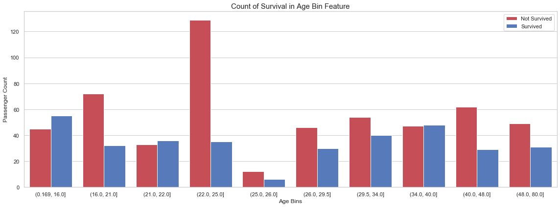
6.6 Age Binning
Similar to the Fare feature, we bin the age feature.
df_all['Age_Bin'] = pd.qcut(df_all['Age'], 10)
fig, axs = plt.subplots(figsize=(16, 6))
sns.countplot(x='Age_Bin', hue='Survived', data=df_all, palette=sns.diverging_palette(10, 255, sep=80, n=2))

plt.xlabel('Age Bins')
plt.ylabel('Passenger Count')
plt.legend(['Not Survived', 'Survived'], loc='upper right')
plt.title('Count of Survival in {} Feature'.format('Age Bin'), size=15)
plt.tight_layout()
6.7 Encoding
In order for our model to interpret categorical and non-numerical features, we need to generate new feature for each possible label.
The following features need to be encoded:
- Embarked
- Sex
- Deck
- Family_Size_Grp
- Age_Bin
- Fare_Bin
- Title
df_train, df_test = divide_df(df_all)
# features to be encoded
encoding = ['Embarked', 'Sex', 'Deck', 'Family_Size_Grp', 'Age_Bin', 'Fare_Bin', 'Title']

for feature in encoding:
    encoder = LabelEncoder()
    df_train[feature] = encoder.fit_transform(df_train[feature])
    df_test[feature] = encoder.transform(df_test[feature])
Once the features have been encoded, we can create dummies.
dummies = ['Pclass', 'Sex', 'Deck', 'Embarked', 'Title', 'Family_Size_Grp']
df_train = pd.get_dummies(df_train, prefix_sep='_', columns=dummies, drop_first=False)
df_test = pd.get_dummies(df_test, prefix_sep='_', columns=dummies, drop_first=False)
Finally, we can drop several columns that we do not need.
df_all = concat_df(df_train, df_test)
drop_columns = ['Family_Size', 'Survived', 'Name', 'Parch', 'Last_Name', 'PassengerId', 'SibSp',
                'Ticket', 'Ticket_Survival', 'Family_Survival', 'Has_Family_Survival', 'Has_Ticket_Survival',
                'Age', 'Fare']

drop_columns_test = ['Family_Size', 'Name', 'Parch', 'Last_Name', 'PassengerId', 'SibSp',
                     'Ticket', 'Ticket_Survival', 'Family_Survival', 'Has_Family_Survival', 'Has_Ticket_Survival',
                     'Age', 'Fare']
df_all = df_all.drop(columns=drop_columns)
df_all.head()
| Age_Bin | Deck_0 | Deck_1 | Deck_2 | Deck_3 | Embarked_0 | Embarked_1 | Embarked_2 | Family_Size_Grp_0 | Family_Size_Grp_1 | ... | Pclass_2 | Pclass_3 | Sex_0 | Sex_1 | Survival_Rate | Ticket_Frequency | Title_0 | Title_1 | Title_2 | Title_3 | |
|---|---|---|---|---|---|---|---|---|---|---|---|---|---|---|---|---|---|---|---|---|---|
| 0 | 2 | 0 | 0 | 0 | 1 | 0 | 0 | 1 | 0 | 0 | ... | 0 | 1 | 0 | 1 | 0.383838 | 1 | 0 | 0 | 1 | 0 |
| 1 | 7 | 1 | 0 | 0 | 0 | 1 | 0 | 0 | 0 | 0 | ... | 0 | 0 | 1 | 0 | 1.000000 | 2 | 0 | 1 | 0 | 0 |
| 2 | 4 | 0 | 0 | 0 | 1 | 0 | 0 | 1 | 1 | 0 | ... | 0 | 1 | 1 | 0 | 0.383838 | 1 | 0 | 1 | 0 | 0 |
| 3 | 7 | 1 | 0 | 0 | 0 | 0 | 0 | 1 | 0 | 0 | ... | 0 | 0 | 1 | 0 | 0.383838 | 2 | 0 | 1 | 0 | 0 |
| 4 | 7 | 0 | 0 | 0 | 1 | 0 | 0 | 1 | 1 | 0 | ... | 0 | 1 | 0 | 1 | 0.383838 | 1 | 0 | 0 | 1 | 0 |
5 rows × 26 columns
df_all.columns
Index(['Age_Bin', 'Deck_0', 'Deck_1', 'Deck_2', 'Deck_3', 'Embarked_0',
       'Embarked_1', 'Embarked_2', 'Family_Size_Grp_0', 'Family_Size_Grp_1',
       'Family_Size_Grp_2', 'Family_Size_Grp_3', 'Fare_Bin', 'Has_Survival',
       'Is_Married', 'Pclass_1', 'Pclass_2', 'Pclass_3', 'Sex_0', 'Sex_1',
       'Survival_Rate', 'Ticket_Frequency', 'Title_0', 'Title_1', 'Title_2',
       'Title_3'],
      dtype='object')
7. Model Preparation
We will now prepare the data before creating a model. The preparation is divided into three steps:
- Separate the dataframe into our input data and our output feature (X and y).
- Normalize the data
X_train = StandardScaler().fit_transform(df_train.drop(columns=drop_columns))
y_train = df_train['Survived'].values
X_test = StandardScaler().fit_transform(df_test.drop(columns=drop_columns_test))

print('X_train shape: {}'.format(X_train.shape))
print('y_train shape: {}'.format(y_train.shape))
print('X_test shape: {}'.format(X_test.shape))
X_train shape: (891, 26)
y_train shape: (891,)
X_test shape: (418, 26)
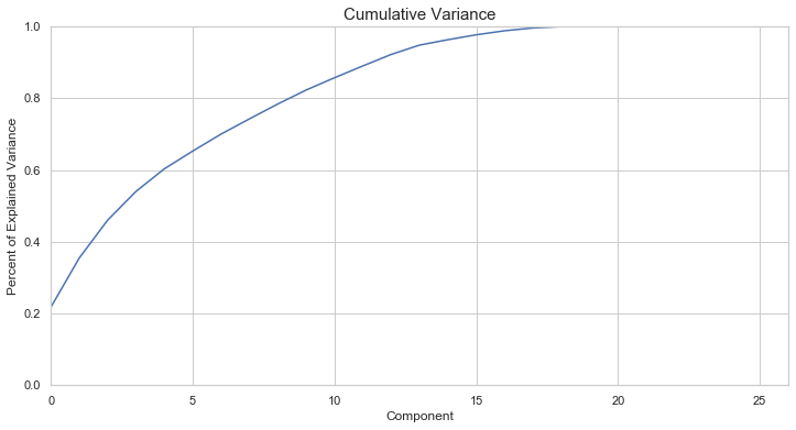
# PCA
pca = PCA(random_state=42)
X_pca = pca.fit_transform(X_train)
fig, ax = plt.subplots(figsize=(12,6))
ax.plot(np.cumsum(pca.explained_variance_ratio_))
ax.set_xlabel("Component")
ax.set_ylabel("Percent of Explained Variance")
ax.set_title("Cumulative Variance", fontsize=15)
ax.set_ylim(0,1)
ax.set_xlim(0,pca.n_components_);
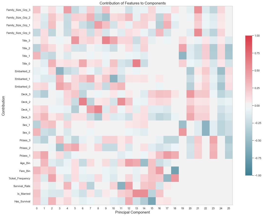
fig, ax = plt.subplots(figsize=(16,16))
cmap = sns.diverging_palette(220, 10, as_cmap=True)
cset = ax.imshow(
    pca.components_.T,
    cmap = cmap,
    vmin=-1,
    vmax=1)

ylabels = df_train.drop(columns=drop_columns).columns.values.tolist()
ax.set_yticks(np.arange(len(ylabels)))
ax.set_yticklabels(ylabels, rotation=0)
ax.set_ylim(-0.5,len(ylabels)-0.5)
ax.set_xticks(range(pca.n_components_))
ax.grid(False)
ax.set_xlabel("Principal Component", fontsize=15)
ax.set_ylabel("Contribution", fontsize=15)
ax.set_title("Contribution of Features to Components", fontsize=15)
fig.colorbar(cset, ax=ax, shrink=0.5)
plt.tight_layout();
8. Models
In this section, we will make predictions using the following models:
- RandomForestClassifier
- ExtraTreesClassifier
- LogisticRegression
- GradientBoostingClassifier
- LinearDiscriminantAnalysis
- RidgeClassifier
- XGBClassifier
- MLPClassifier
- BaggingClassifier
- BernoulliNB
- ExtraTreeClassifier
- DecisionTreeClassifier
- LinearSVC
- AdaBoostClassifier
- SVC
- NuSVC
- SGDClassifier
- Perceptron
- GaussianProcessClassifier
- KNeighborsClassifier
- GaussianNB
- PassiveAggressiveClassifier
- QuadraticDiscriminantAnalysis
# Cross validate model with Kfold stratified cross val
kfold = StratifiedKFold(n_splits=5, random_state=5, shuffle=True)
random_state = 42
# classifiers
classifiers_list = [
    #Ensemble Methods
    AdaBoostClassifier(AdaBoostClassifier(DecisionTreeClassifier(random_state=random_state),random_state=random_state)),
    BaggingClassifier(random_state=random_state),
    ExtraTreesClassifier(random_state=random_state),
    GradientBoostingClassifier(random_state=random_state),
    RandomForestClassifier(random_state=random_state),

    #Gaussian Processes
    GaussianProcessClassifier(random_state=random_state),

    #GLM
    LogisticRegression(random_state=random_state),
    PassiveAggressiveClassifier(random_state=random_state),
    RidgeClassifier(),
    SGDClassifier(random_state=random_state),
    Perceptron(random_state=random_state),
    MLPClassifier(random_state=random_state),

    #Navies Bayes
    BernoulliNB(),
    GaussianNB(),

    #Nearest Neighbor
    KNeighborsClassifier(),

    #SVM
    SVC(probability=True, random_state=random_state),
    NuSVC(probability=True, random_state=random_state),
    LinearSVC(random_state=random_state),

    #Trees
    DecisionTreeClassifier(random_state=random_state),
    ExtraTreeClassifier(random_state=random_state),

    #Discriminant Analysis
    LinearDiscriminantAnalysis(),
    QuadraticDiscriminantAnalysis(),

    #xgboost: http://xgboost.readthedocs.io/en/latest/model.html
    XGBClassifier()
    ]

# store cv results in list
cv_results_list = []
cv_means_list = []
cv_std_list = []

# perform cross-validation
for clf in tqdm(classifiers_list):
    cv_results_list.append(cross_val_score(clf,
                                           X_train,
                                           y_train,
                                           scoring = "accuracy",
                                           cv = kfold,
                                           n_jobs=-1))
    clf.fit(X_train, y_train)
    pred = clf.predict(X_test)

# store mean and std accuracy
for cv_result in cv_results_list:
    cv_means_list.append(cv_result.mean())
    cv_std_list.append(cv_result.std())

cv_res_df = pd.DataFrame({"CrossValMeans":cv_means_list,
                          "CrossValerrors": cv_std_list,
                          "Algorithm":[clf.__class__.__name__ for clf in classifiers_list]})

cv_res_df = cv_res_df.sort_values(by='CrossValMeans',ascending=False)
100%|██████████████████████████████████████████████████████████████████████████████████| 23/23 [00:20<00:00, 1.12it/s]
cv_res_df.set_index('Algorithm')
| CrossValMeans | CrossValerrors | |
|---|---|---|
| Algorithm | ||
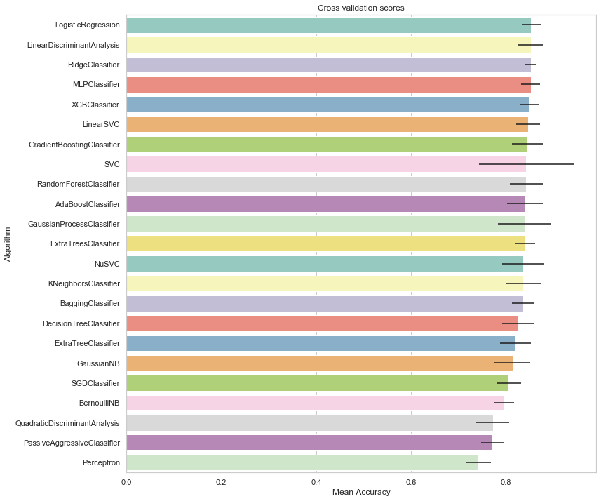
| LogisticRegression | 0.853035 | 0.035074 |
| GradientBoostingClassifier | 0.853010 | 0.028286 |
| LinearDiscriminantAnalysis | 0.851893 | 0.026919 |
| RidgeClassifier | 0.851893 | 0.026919 |
| LinearSVC | 0.850781 | 0.030352 |
| MLPClassifier | 0.850769 | 0.026927 |
| XGBClassifier | 0.850769 | 0.027849 |
| NuSVC | 0.840675 | 0.028222 |
| SVC | 0.840669 | 0.028718 |
| SGDClassifier | 0.837261 | 0.028204 |
| GaussianProcessClassifier | 0.835057 | 0.026180 |
| RandomForestClassifier | 0.831674 | 0.023097 |
| KNeighborsClassifier | 0.829452 | 0.027523 |
| BaggingClassifier | 0.823828 | 0.026461 |
| ExtraTreesClassifier | 0.821581 | 0.026906 |
| AdaBoostClassifier | 0.818204 | 0.028622 |
| DecisionTreeClassifier | 0.810345 | 0.019053 |
| GaussianNB | 0.808123 | 0.032538 |
| ExtraTreeClassifier | 0.805850 | 0.016329 |
| BernoulliNB | 0.795750 | 0.011812 |
| Perceptron | 0.766675 | 0.060092 |
| QuadraticDiscriminantAnalysis | 0.754234 | 0.024949 |
| PassiveAggressiveClassifier | 0.727224 | 0.068009 |
# plot results
fig, ax = plt.subplots(figsize=(12,12))
g = sns.barplot("CrossValMeans",
                "Algorithm",
                data = cv_res_df,
                palette="Set3",
                orient = "h",
                **{'xerr':cv_std_list})
g.set_xlabel("Mean Accuracy")
g = g.set_title("Cross validation scores")
# store best models
best_models = []
def optimize_model(model, X_train, y_train, paramgrid, random_state=10, suffix='_best',
                  metric = 'accuracy', kfold=StratifiedKFold(n_splits=5, random_state=5, shuffle=True), verbose=1, other_args={}, print_best=True):

    # adjust base estimator parameters
    estimator = model(**other_args)

    # create k-fold-based grid-search
    gridsearch = GridSearchCV(estimator, param_grid=paramgrid, cv=kfold, scoring=metric, n_jobs=-1, verbose=verbose)

    # fit grid search
    gridsearch.fit(X_train, y_train)

    # store best model
    name = model.__name__ + suffix
    best_models.append((name, gridsearch.best_estimator_))

    # print (optional)
    if print_best:
        print(gridsearch)

    # display accuracy
    print('Best {} model archieves {:.2f}% {}'.format(model.__name__, 100 * gridsearch.best_score_, metric))
param_grid = {
    'max_depth': [3, 5, 6, 7],
    'learning_rate': [0.01, 0.025, 0.05, 0.075, 0,1, 0,15, 0.2],
    'n_estimators': [500, 1000, 1500],
}

optimize_model(XGBClassifier, X_train, y_train, paramgrid=param_grid)
Fitting 5 folds for each of 108 candidates, totalling 540 fits


[Parallel(n_jobs=-1)]: Using backend LokyBackend with 8 concurrent workers.
[Parallel(n_jobs=-1)]: Done  34 tasks      | elapsed:   15.3s
[Parallel(n_jobs=-1)]: Done 184 tasks      | elapsed:  1.3min
[Parallel(n_jobs=-1)]: Done 434 tasks      | elapsed:  2.9min
[Parallel(n_jobs=-1)]: Done 540 out of 540 | elapsed:  3.5min finished


GridSearchCV(cv=StratifiedKFold(n_splits=5, random_state=5, shuffle=True),
             error_score=nan,
             estimator=XGBClassifier(base_score=0.5, booster='gbtree',
                                     colsample_bylevel=1, colsample_bynode=1,
                                     colsample_bytree=1, gamma=0,
                                     learning_rate=0.1, max_delta_step=0,
                                     max_depth=3, min_child_weight=1,
                                     missing=None, n_estimators=100, n_jobs=1,
                                     nthread=None, objective='binary:logistic',
                                     random_state=0, reg_alpha=0, reg_lambda=1,
                                     scale_pos_weight=1, seed=None, silent=None,
                                     subsample=1, verbosity=1),
             iid='deprecated', n_jobs=-1,
             param_grid={'learning_rate': [0.01, 0.025, 0.05, 0.075, 0, 1, 0,
                                           15, 0.2],
                         'max_depth': [3, 5, 6, 7],
                         'n_estimators': [500, 1000, 1500]},
             pre_dispatch='2*n_jobs', refit=True, return_train_score=False,
             scoring='accuracy', verbose=1)
Best XGBClassifier model archieves 85.64% accuracy
param_grid = {
    "max_depth": [None],
    "max_features": [5, 7, 'auto'],
    "min_samples_split": [4, 5, 6],
    "min_samples_leaf": [4, 5, 6],
    "bootstrap": [False],
    "n_estimators": [1500, 2000],
    "criterion": ["gini"]
}

optimize_model(ExtraTreesClassifier, X_train, y_train, paramgrid=param_grid)
Fitting 5 folds for each of 54 candidates, totalling 270 fits


[Parallel(n_jobs=-1)]: Using backend LokyBackend with 8 concurrent workers.
[Parallel(n_jobs=-1)]: Done  34 tasks      | elapsed:   18.5s
[Parallel(n_jobs=-1)]: Done 184 tasks      | elapsed:  1.5min
[Parallel(n_jobs=-1)]: Done 270 out of 270 | elapsed:  2.3min finished


GridSearchCV(cv=StratifiedKFold(n_splits=5, random_state=5, shuffle=True),
             error_score=nan,
             estimator=ExtraTreesClassifier(bootstrap=False, ccp_alpha=0.0,
                                            class_weight=None, criterion='gini',
                                            max_depth=None, max_features='auto',
                                            max_leaf_nodes=None,
                                            max_samples=None,
                                            min_impurity_decrease=0.0,
                                            min_impurity_split=None,
                                            min_samples_leaf=1,
                                            min_samples_split=2,
                                            min_w...
                                            oob_score=False, random_state=None,
                                            verbose=0, warm_start=False),
             iid='deprecated', n_jobs=-1,
             param_grid={'bootstrap': [False], 'criterion': ['gini'],
                         'max_depth': [None], 'max_features': [5, 7, 'auto'],
                         'min_samples_leaf': [4, 5, 6],
                         'min_samples_split': [4, 5, 6],
                         'n_estimators': [1500, 2000]},
             pre_dispatch='2*n_jobs', refit=True, return_train_score=False,
             scoring='accuracy', verbose=1)
Best ExtraTreesClassifier model archieves 83.96% accuracy
param_grid = {
    "max_depth": [5, 6, 7],
    "min_samples_split": [4, 5, 6],
    "min_samples_leaf": [4, 5, 6],
    "max_features": [5, 7, 'auto'],
    "n_estimators": [1750],
    "criterion": ["gini"]
}

optimize_model(RandomForestClassifier, X_train, y_train, paramgrid=param_grid)
Fitting 5 folds for each of 81 candidates, totalling 405 fits


[Parallel(n_jobs=-1)]: Using backend LokyBackend with 8 concurrent workers.
[Parallel(n_jobs=-1)]: Done  34 tasks      | elapsed:   29.4s
[Parallel(n_jobs=-1)]: Done 184 tasks      | elapsed:  2.0min
[Parallel(n_jobs=-1)]: Done 405 out of 405 | elapsed:  4.3min finished


GridSearchCV(cv=StratifiedKFold(n_splits=5, random_state=5, shuffle=True),
             error_score=nan,
             estimator=RandomForestClassifier(bootstrap=True, ccp_alpha=0.0,
                                              class_weight=None,
                                              criterion='gini', max_depth=None,
                                              max_features='auto',
                                              max_leaf_nodes=None,
                                              max_samples=None,
                                              min_impurity_decrease=0.0,
                                              min_impurity_split=None,
                                              min_samples_leaf=1,
                                              min_samples_split=2,
                                              min_...
                                              n_estimators=100, n_jobs=None,
                                              oob_score=False,
                                              random_state=None, verbose=0,
                                              warm_start=False),
             iid='deprecated', n_jobs=-1,
             param_grid={'criterion': ['gini'], 'max_depth': [5, 6, 7],
                         'max_features': [5, 7, 'auto'],
                         'min_samples_leaf': [4, 5, 6],
                         'min_samples_split': [4, 5, 6],
                         'n_estimators': [1750]},
             pre_dispatch='2*n_jobs', refit=True, return_train_score=False,
             scoring='accuracy', verbose=1)
Best RandomForestClassifier model archieves 84.74% accuracy
param_grid = {
    'kernel': ['rbf'],
    'gamma': [0.0005, 0.0008, 0.001, 0.005, 0.01, 0.05, 0.1, 0.5, 1],
    'C': [1, 10, 50, 100, 200, 250, 500]
}

optimize_model(SVC, X_train, y_train, paramgrid=param_grid, other_args={'probability':True})
Fitting 5 folds for each of 63 candidates, totalling 315 fits


[Parallel(n_jobs=-1)]: Using backend LokyBackend with 8 concurrent workers.
[Parallel(n_jobs=-1)]: Done  52 tasks      | elapsed:    0.8s
[Parallel(n_jobs=-1)]: Done 300 out of 315 | elapsed:    9.5s remaining:    0.4s


GridSearchCV(cv=StratifiedKFold(n_splits=5, random_state=5, shuffle=True),
             error_score=nan,
             estimator=SVC(C=1.0, break_ties=False, cache_size=200,
                           class_weight=None, coef0=0.0,
                           decision_function_shape='ovr', degree=3,
                           gamma='scale', kernel='rbf', max_iter=-1,
                           probability=True, random_state=None, shrinking=True,
                           tol=0.001, verbose=False),
             iid='deprecated', n_jobs=-1,
             param_grid={'C': [1, 10, 50, 100, 200, 250, 500],
                         'gamma': [0.0005, 0.0008, 0.001, 0.005, 0.01, 0.05,
                                   0.1, 0.5, 1],
                         'kernel': ['rbf']},
             pre_dispatch='2*n_jobs', refit=True, return_train_score=False,
             scoring='accuracy', verbose=1)
Best SVC model archieves 85.42% accuracy


[Parallel(n_jobs=-1)]: Done 315 out of 315 | elapsed:   10.2s finished
param_grid = {"C": np.logspace(-3, 3, 40), "penalty": ["l1", "l2"]}

optimize_model(LogisticRegression, X_train, y_train, paramgrid=param_grid)
Fitting 5 folds for each of 80 candidates, totalling 400 fits


[Parallel(n_jobs=-1)]: Using backend LokyBackend with 8 concurrent workers.
[Parallel(n_jobs=-1)]: Done  56 tasks      | elapsed:    0.0s


GridSearchCV(cv=StratifiedKFold(n_splits=5, random_state=5, shuffle=True),
             error_score=nan,
             estimator=LogisticRegression(C=1.0, class_weight=None, dual=False,
                                          fit_intercept=True,
                                          intercept_scaling=1, l1_ratio=None,
                                          max_iter=100, multi_class='auto',
                                          n_jobs=None, penalty='l2',
                                          random_state=None, solver='lbfgs',
                                          tol=0.0001, verbose=0,
                                          warm_start=False),
             iid='deprecated'...
       4.92388263e+00, 7.01703829e+00, 1.00000000e+01, 1.42510267e+01,
       2.03091762e+01, 2.89426612e+01, 4.12462638e+01, 5.87801607e+01,
       8.37677640e+01, 1.19377664e+02, 1.70125428e+02, 2.42446202e+02,
       3.45510729e+02, 4.92388263e+02, 7.01703829e+02, 1.00000000e+03]),
                         'penalty': ['l1', 'l2']},
             pre_dispatch='2*n_jobs', refit=True, return_train_score=False,
             scoring='accuracy', verbose=1)
Best LogisticRegression model archieves 85.64% accuracy


[Parallel(n_jobs=-1)]: Done 400 out of 400 | elapsed:    0.3s finished
param_grid = {
    "learning_rate": [0.01, 0.025, 0.05, 0.075, 0.1, 0.15, 0.2],
    "subsample": [0.5, 0.62, 0.8, 0.85, 0.87, 0.9, 0.95, 1.0]
}

optimize_model(GradientBoostingClassifier,
               X_train,
               y_train,
               paramgrid=param_grid)
[Parallel(n_jobs=-1)]: Using backend LokyBackend with 8 concurrent workers.


Fitting 5 folds for each of 56 candidates, totalling 280 fits


[Parallel(n_jobs=-1)]: Done  52 tasks      | elapsed:    1.5s


GridSearchCV(cv=StratifiedKFold(n_splits=5, random_state=5, shuffle=True),
             error_score=nan,
             estimator=GradientBoostingClassifier(ccp_alpha=0.0,
                                                  criterion='friedman_mse',
                                                  init=None, learning_rate=0.1,
                                                  loss='deviance', max_depth=3,
                                                  max_features=None,
                                                  max_leaf_nodes=None,
                                                  min_impurity_decrease=0.0,
                                                  min_impurity_split=None,
                                                  min_samples_leaf=1,
                                                  min_samples_split=2,
                                                  min...
                                                  n_iter_no_change=None,
                                                  presort='deprecated',
                                                  random_state=None,
                                                  subsample=1.0, tol=0.0001,
                                                  validation_fraction=0.1,
                                                  verbose=0, warm_start=False),
             iid='deprecated', n_jobs=-1,
             param_grid={'learning_rate': [0.01, 0.025, 0.05, 0.075, 0.1, 0.15,
                                           0.2],
                         'subsample': [0.5, 0.62, 0.8, 0.85, 0.87, 0.9, 0.95,
                                       1.0]},
             pre_dispatch='2*n_jobs', refit=True, return_train_score=False,
             scoring='accuracy', verbose=1)
Best GradientBoostingClassifier model archieves 86.20% accuracy


[Parallel(n_jobs=-1)]: Done 280 out of 280 | elapsed:    6.8s finished
param_grid = {
    "n_neighbors": [3, 5, 7, 11, 13, 15],
    "weights": ['uniform', 'distance'],
    "metric": ['manhattan'],
    "algorithm":['auto']
}

optimize_model(KNeighborsClassifier,
               X_train,
               y_train,
               paramgrid=param_grid)
Fitting 5 folds for each of 12 candidates, totalling 60 fits


[Parallel(n_jobs=-1)]: Using backend LokyBackend with 4 concurrent workers.


GridSearchCV(cv=StratifiedKFold(n_splits=5, random_state=5, shuffle=True),
             error_score='raise-deprecating',
             estimator=KNeighborsClassifier(algorithm='auto', leaf_size=30,
                                            metric='minkowski',
                                            metric_params=None, n_jobs=None,
                                            n_neighbors=5, p=2,
                                            weights='uniform'),
             iid='warn', n_jobs=-1,
             param_grid={'algorithm': ['auto'], 'metric': ['manhattan'],
                         'n_neighbors': [3, 5, 7, 11, 13, 15],
                         'weights': ['uniform', 'distance']},
             pre_dispatch='2*n_jobs', refit=True, return_train_score=False,
             scoring='accuracy', verbose=1)
Best KNeighborsClassifier model archieves 83.95% accuracy


[Parallel(n_jobs=-1)]: Done  60 out of  60 | elapsed:    4.1s finished
LDA = LinearDiscriminantAnalysis()
LDA.fit(X_train, y_train)
LDA_best = LDA
best_models.append(("LDA_best", LDA_best))
predictions = {}
N_fold = 5


def generalize_predictions(model,
                           X_train,
                           y_train,
                           X_test,
                           skf=StratifiedKFold(n_splits=N_fold,
                                               random_state=N_fold,
                                               shuffle=True)):

    # store predicted probas for each folds
    probas = pd.DataFrame(np.zeros((len(X_test), N_fold * 2)),
                          columns=[
                              'Fold_{}_Class_{}'.format(i, j)
                              for i in range(1, N_fold + 1) for j in range(2)
                          ],
                          index=passengerId)

    # for each fold, train then predict
    for fold_id, (train_idx,
                  val_idx) in tqdm(enumerate(skf.split(X_train, y_train), 1)):

        # Fitting the model
        model.fit(X_train[train_idx], y_train[train_idx])

        # X_test probabilities
        probas.loc[:, 'Fold_{}_Class_0'.format(fold_id)] = model.predict_proba(
            X_test)[:, 0]
        probas.loc[:, 'Fold_{}_Class_1'.format(fold_id)] = model.predict_proba(
            X_test)[:, 1]

    # save results
    return (probas)
predictions = {name: generalize_predictions(model, X_train, y_train, X_test) for name, model in best_models}
5it [00:07,  1.49s/it]
5it [00:13,  2.70s/it]
5it [00:13,  2.78s/it]
5it [00:01,  3.91it/s]
5it [00:00, 40.15it/s]
5it [00:00,  6.12it/s]
5it [00:00, 18.64it/s]
5it [00:00, 116.72it/s]
def make_predictions(model_df, mode="hard", threshold=0.5):

    predictions = pd.DataFrame(np.zeros((len(X_test), 3)),
                     columns=['1', '0', 'pred'])

    # isolate probabilities of class 1
    class_one = [col for col in model_df.columns if col.endswith('Class_1')]

    # compute average of class 1 probabilities
    predictions['1'] = model_df[class_one].sum(axis=1) / N_fold
    predictions['0'] = 1. - predictions['1']

    if mode=="hard":
        predictions['pred'] = (predictions['1'] >= threshold).astype(int)
    else:
        predictions['pred'] = predictions['1']

    model_results = pd.DataFrame(columns=['PassengerId', 'Survived'])
    model_results['PassengerId'] = df_test['PassengerId']
    model_results['Survived'] = predictions['pred']
    return model_results
results = [(key, make_predictions(model)) for key, model in predictions.items()]
9. Best Models
for name, model in best_models:
    print(name)
XGBClassifier_best
ExtraTreesClassifier_best
RandomForestClassifier_best
SVC_best
LogisticRegression_best
GradientBoostingClassifier_best
KNeighborsClassifier_best
LDA_best
predictions = []

for model_name, model in tqdm(best_models):
    # make predictions
    y_pred = model.predict(X_test)

    # store predictions
    predictions.append(pd.Series(y_pred, name=model_name))

# concatenate predictions
ensemble_results = pd.concat(predictions, axis=1)
100%|██████████| 8/8 [00:00<00:00, 16.13it/s]
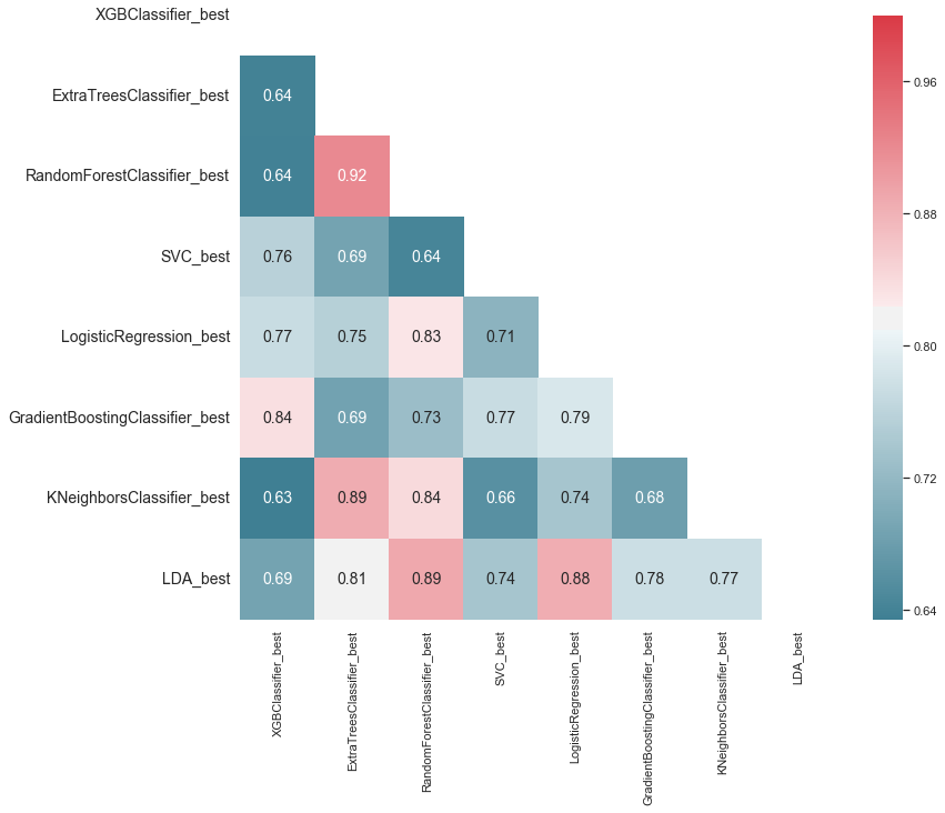
# Generate a mask for the upper triangle
mask = np.zeros_like(ensemble_results.corr(), dtype=np.bool)
mask[np.triu_indices_from(mask)] = True

fig, ax = plt.subplots(figsize=(12, 10))

cmap = sns.diverging_palette(220, 10, as_cmap=True)

g = sns.heatmap(ensemble_results.corr(),
                annot=True,
                mask=mask,
                annot_kws={"fontsize": 14}, cmap=cmap)

ylabels = [x.get_text() for x in g.get_yticklabels()]
plt.yticks(np.arange(len(ylabels)) + 0.5,
           ylabels,
           rotation=0,
           fontsize="14",
           va="center")
g.set_ylim(len(best_models), 0.5);
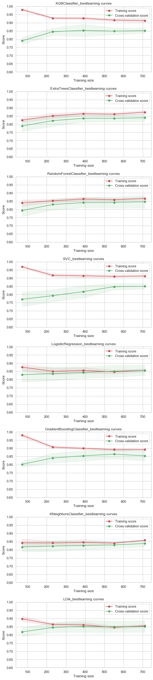
def plot_learning_curve(models,
                        X,
                        y,
                        ylim=None,
                        cv=None,
                        n_jobs=-1,
                        train_sizes=np.linspace(.1, 1.0, 5)):

    # extract number of models
    n_models = len(models)

    # create figure
    fix, axes = plt.subplots(n_models, 1, figsize=(8, 5 * n_models))

    for idx, val in enumerate(models):
        # unpack
        name, model = val

        # scale y axis
        if ylim is not None: axes[idx].set_ylim(*ylim)
        # set title
        axes[idx].set_title(name + "learning curves")
        # set labels
        axes[idx].set_xlabel("Training size")
        axes[idx].set_ylabel("Score")
        # compute learning curves
        train_sizes, train_scores, test_scores = learning_curve(
            model, X, y, cv=cv, n_jobs=n_jobs, train_sizes=train_sizes)
        # compute statistics
        train_score_mean = np.mean(train_scores, axis=1)
        train_score_std = np.std(train_scores, axis=1)
        test_score_mean = np.mean(test_scores, axis=1)
        test_score_std = np.std(test_scores, axis=1)

        axes[idx].fill_between(train_sizes,
                               train_score_mean - train_score_std,
                               train_score_mean + train_score_std,
                               alpha=0.1,
                               color='r')
        axes[idx].fill_between(train_sizes,
                               test_score_mean - test_score_std,
                               test_score_mean + test_score_std,
                               alpha=0.1,
                               color='g')

        axes[idx].plot(train_sizes,
                       train_score_mean,
                       'o-',
                       color="r",
                       label="Training score")
        axes[idx].plot(train_sizes,
                       test_score_mean,
                       'o-',
                       color="g",
                       label="Cross-validation score")
        axes[idx].legend(loc='best')

    plt.subplots_adjust(hspace=0.3)
    return fig, axes
plot_learning_curve(best_models,X_train,y_train,cv=kfold, ylim=(0.6,1.));
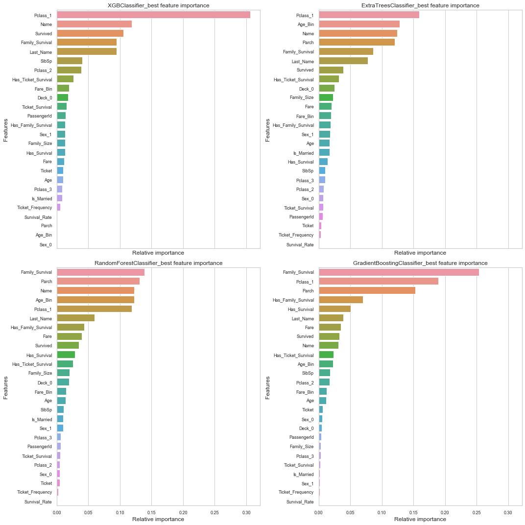
nrows = ncols = 2
fig, axes = plt.subplots(nrows = nrows, ncols = ncols, sharex="all", figsize=(15,15))

names_classifiers = [("XGBClassifier_best",best_models[0][1]),
                     ("ExtraTreesClassifier_best",best_models[1][1]),
                     ("RandomForestClassifier_best",best_models[2][1]),
                     ("GradientBoostingClassifier_best",best_models[5][1])]

nclassifier = 0
for row in range(nrows):
    for col in range(ncols):
        name = names_classifiers[nclassifier][0]
        classifier = names_classifiers[nclassifier][1]
        indices = np.argsort(classifier.feature_importances_)[::-1][:40]
        g = sns.barplot(y=df_train.columns[indices][:40],x = classifier.feature_importances_[indices][:40] , orient='h',ax=axes[row][col])
        g.set_xlabel("Relative importance",fontsize=12)
        g.set_ylabel("Features",fontsize=12)
        g.tick_params(labelsize=9)
        g.set_title(name + " feature importance")
        nclassifier += 1
plt.tight_layout()
10. Create Submission
# generate submission file
submission_df = pd.DataFrame({'PassengerId': passengerId,
                            'Survived': results[2][1].values.T[0]})
submission_df.to_csv("voting_submission_df.csv", index=False)
The submission leads to a 81.339% accuracy. This is puts the predictions in the top 3% of the Kaggle leaderboard.