New Veterinary Clinic in Toronto

credit: https://www.uplacevet.com/
Table of Content
- Introduction
- Load Tools
- Data Import 3.a. Census Data
3.b. Animal Registry
3.c. Toronto Neighborhoods - Data Cleaning and Combination 4.a. Neighborhood
4.b. Census Data
4.c Animal Registry
4.d Final Filtering - Existing Veterinarians
- Feature Engineering
- Exploration and Analysis
7.a. Population Distribution
7.b. Animal Distribution
7.c. Change in Animal Registration
7.d. Vet distribution
7.e. Cat vs Dog Friendly Neighborhoods
7.f. Feature correlations - Clustering
1. Introduction
As a consultant specialized in helping new businesses to start in the Toronto area, we are often required to look at the status of the current market to provide valuable advice to our client. In this case, we were contacted to perform a survey of the veterinarian market in the city of Toronto. Our client wants to find us to recommend a good candidate neighborhood to start open their veterinarian clinic.
Our analysis will be divided into the following phases:
- Gather data
- Get useful insights of the current status of the vet market
- Leverage machine learning technique to identify areas lacking veterinarians
HERE IS A LIKE TO THE FINAL REPORT: Here
2. Load Tools
In this section, we load the libraries that we will be using during this project.
# data structures
print('Loading....')
import numpy as np
print('\tnumpy:\t\t',np.__version__)
import pandas as pd
print('\tpandas:\t\t',pd.__version__)
pd.set_option('display.max_rows', 500)
pd.set_option('display.max_columns', 500)
pd.set_option('display.width', 1000)
# plot libraries
import matplotlib
print('\tmatplotlib:\t',matplotlib.__version__)
import matplotlib.pyplot as plt
import matplotlib.cm as cm
import matplotlib.colors as colors
import seaborn as sns
print('\tseaborn:\t',sns.__version__)
plt.style.use('ggplot')
# geolocalization
import folium
print('\tfolium:\t\t',folium.__version__)
import geocoder
print('\tgeocoder:\t',geocoder.__version__)
from geopy.geocoders import Nominatim
# url fetch
import requests
print('\trequests:\t',requests.__version__)
from pandas.io.json import json_normalize
# scrapping
import bs4
from bs4 import BeautifulSoup
print('\tbs4:\t\t',bs4.__version__)
# python
import warnings
warnings.simplefilter(action='ignore', category=FutureWarning)
# sklearn
import sklearn
print('\tsklearn:\t',sklearn.__version__)
from sklearn.preprocessing import StandardScaler
from sklearn.cluster import KMeans
Loading....
numpy: 1.16.2
pandas: 0.24.1
matplotlib: 3.0.2
seaborn: 0.9.0
folium: 0.8.0
geocoder: 1.38.1
requests: 2.18.4
bs4: 4.6.0
sklearn: 0.19.1
3. Data Import
3.a. Census Data
The census data is retrieved from the database made available by the city of Toronto.
The census data dated from 2016 is used. It is loaded as a *.csv file.
https://www12.statcan.gc.ca/census-recensement/2016/dp-pd/hlt-fst/pd-pl/comprehensive.cfm
# URL to CSV from the governement of Canada: FSA census of 2016
print('Loading census data...')
URL_census = 'https://www12.statcan.gc.ca/census-recensement/2016/dp-pd/hlt-fst/pd-pl/Tables/CompFile.cfm?Lang=Eng&T=1201&OFT=FULLCSV'
print('...Census data loaded')
Loading census data...
...Census data loaded
We inspect the head of the dataframe in order to determine what features are contained in the dataset.
df_census_raw = pd.read_csv(URL_census)
df_census_raw.head()
| Geographic code | Geographic name | Province or territory | Incompletely enumerated Indian reserves and Indian settlements, 2016 | Population, 2016 | Total private dwellings, 2016 | Private dwellings occupied by usual residents, 2016 | |
|---|---|---|---|---|---|---|---|
| 0 | 01 | Canada | NaN | T | 35151728.0 | 15412443.0 | 14072079.0 |
| 1 | A0A | A0A | Newfoundland and Labrador | NaN | 46587.0 | 26155.0 | 19426.0 |
| 2 | A0B | A0B | Newfoundland and Labrador | NaN | 19792.0 | 13658.0 | 8792.0 |
| 3 | A0C | A0C | Newfoundland and Labrador | NaN | 12587.0 | 8010.0 | 5606.0 |
| 4 | A0E | A0E | Newfoundland and Labrador | NaN | 22294.0 | 12293.0 | 9603.0 |
We inspect the properties of the dataset using the .info() function and .shape attribute.
df_census_raw.info()
<class 'pandas.core.frame.DataFrame'>
RangeIndex: 1648 entries, 0 to 1647
Data columns (total 7 columns):
Geographic code 1648 non-null object
Geographic name 1643 non-null object
Province or territory 1641 non-null object
Incompletely enumerated Indian reserves and Indian settlements, 2016 1 non-null object
Population, 2016 1642 non-null float64
Total private dwellings, 2016 1642 non-null float64
Private dwellings occupied by usual residents, 2016 1642 non-null float64
dtypes: float64(3), object(4)
memory usage: 90.2+ KB
The next step is to look at missing and null values. We count how many values are null for each feature.
df_census_raw.isna().sum(axis=0)
Geographic code 0
Geographic name 5
Province or territory 7
Incompletely enumerated Indian reserves and Indian settlements, 2016 1647
Population, 2016 6
Total private dwellings, 2016 6
Private dwellings occupied by usual residents, 2016 6
dtype: int64
print("The census data contains {} rows and {} columns.".format(df_census_raw.shape[0],df_census_raw.shape[1]))
The census data contains 1648 rows and 7 columns.
We remove columns that are not meant to be used in this study, we keep:
- Geographic code
- Population, 2016
- Private dwellings occupied by usual residents, 2016
Note: we only keep the population and the dwelling count features from the census data.
df_census_raw = df_census_raw[['Geographic code','Population, 2016','Private dwellings occupied by usual residents, 2016']]
df_census_raw.head()
| Geographic code | Population, 2016 | Private dwellings occupied by usual residents, 2016 | |
|---|---|---|---|
| 0 | 01 | 35151728.0 | 14072079.0 |
| 1 | A0A | 46587.0 | 19426.0 |
| 2 | A0B | 19792.0 | 8792.0 |
| 3 | A0C | 12587.0 | 5606.0 |
| 4 | A0E | 22294.0 | 9603.0 |
3.b. Animal Registry
The city of Toronto website contains the cat and dog registry for the years 2013 through 2017.
https://www.toronto.ca/ext/open_data/catalog/data_set_files/2017_dog_and_cat_licence_FSA.xls
https://www.toronto.ca/ext/open_data/catalog/data_set_files/2013%20licences%20sold%20by%20fsa.xls
# URL of the XLS files
URL_2017 = 'https://www.toronto.ca/ext/open_data/catalog/data_set_files/2017_dog_and_cat_licence_FSA.xls'
URL_2013 = 'https://www.toronto.ca/ext/open_data/catalog/data_set_files/2013%20licences%20sold%20by%20fsa.xls'
URL_animal = [URL_2013,URL_2017]
# load all the XLS files
list_df = []
list_skiprows = [3,2,2,2,2]
list_skip_footer = [1,1,0,0,1]
# create list of DataFrame
print('Loading census data...')
for idx,url in enumerate(URL_animal):
df = pd.read_excel(url,sheet_name='Sheet1',skiprows=list_skiprows[idx],skipfooter=list_skip_footer[idx])
df.columns = ['FSA','CAT','DOG','TOTAL']
df['Year'] = idx*4+2013
list_df.append(df)
print('...Animal registration data loaded.')
Loading census data...
...Animal registration data loaded.
Let’s print the shape of the dataframe and explore the nature of its features.
# combine the dataFrames
df_animals = list_df[0].merge(list_df[1],on='FSA',suffixes=('_2013','_2017'))
print("The animal registry data contains {} rows and {} columns.".format(df_animals.shape[0],df_animals.shape[1]))
The animal registry data contains 97 rows and 9 columns.
print('Dataset info:')
print(' ')
df_animals.info()
Dataset info:
<class 'pandas.core.frame.DataFrame'>
Int64Index: 97 entries, 0 to 96
Data columns (total 9 columns):
FSA 97 non-null object
CAT_2013 97 non-null int64
DOG_2013 97 non-null int64
TOTAL_2013 97 non-null int64
Year_2013 97 non-null int64
CAT_2017 97 non-null int64
DOG_2017 97 non-null int64
TOTAL_2017 97 non-null int64
Year_2017 97 non-null int64
dtypes: int64(8), object(1)
memory usage: 7.6+ KB
df_animals = df_animals.drop(['Year_2013','Year_2017'],axis=1)
df_animals.head()
| FSA | CAT_2013 | DOG_2013 | TOTAL_2013 | CAT_2017 | DOG_2017 | TOTAL_2017 | |
|---|---|---|---|---|---|---|---|
| 0 | M1B | 293 | 674 | 967 | 285 | 627 | 912 |
| 1 | M1C | 387 | 967 | 1354 | 297 | 775 | 1072 |
| 2 | M1E | 536 | 1085 | 1621 | 467 | 963 | 1430 |
| 3 | M1G | 252 | 457 | 709 | 220 | 385 | 605 |
| 4 | M1H | 184 | 361 | 545 | 155 | 309 | 464 |
Note: We keep the data as is for now. We will combine the number of animals per neighborhood late.
3.c. Toronto Neighborhoods
3.c.1 Wikipedia Scrapping
The Toronto neighborhoods are retrieved from the Wikipedia page:
https://en.wikipedia.org/wiki/List_of_postal_codes_of_Canada:_M
In this section, we use the BeautifulSoup library to extract the table containing the list of Neighborhood in Toronto. The following steps are followed:
- Create a soup object that contains the webpage data.
- Retrieve the subset of HTML code which contains the table data.
- Extract the headers from the table.
- Extract the content of the table.
Step 1: Create a soup object that contains the webpage data.
# url to be scrapped
URL_toronto = 'https://en.wikipedia.org/wiki/List_of_postal_codes_of_Canada:_M'
# GET request
request = requests.get(URL_toronto)
data = request.text
# convert request to soup
soup = BeautifulSoup(data, "lxml")
print('BeautifulSoup created...')
BeautifulSoup created...
Step 2: Retrieve the subset of HTML code which contains the table data.
# extract the table
match = soup.find('table',class_='wikitable sortable')
print('Table found...')
Table found...
Step 3: Extract the headers from the table.
# create new dataframe used to store the table data
df_toronto_postal = pd.DataFrame(columns=['PostalCode', 'Borough', 'Neighborhood'])
print('DataFrame instantiated...')
DataFrame instantiated...
Step 4: Extract the content of the table.
# fetch table rows tr
data_rows = soup.find('table',class_='wikitable sortable').find('tbody').find_all('tr')
# fetch table cells td
for data_row in data_rows:
data_split = data_row.find_all('td')
if len(data_split)>0:
postcode = data_split[0].text.strip()
borough = data_split[1].text.strip()
neighborhood = data_split[2].text.strip()
df_toronto_postal = df_toronto_postal.append({'PostalCode':postcode,
'Borough':borough,
'Neighborhood':neighborhood},ignore_index=True)
print('DataFrame populated...')
DataFrame populated...
print("The neighborhood database contains {} rows and {} columns.".format(df_toronto_postal.shape[0],df_toronto_postal.shape[1]))
The neighborhood database contains 289 rows and 3 columns.
Let’s print the shape of the dataframe and explore the nature of its features.
print('Dataset info:')
print(' ')
df_toronto_postal.info()
Dataset info:
<class 'pandas.core.frame.DataFrame'>
RangeIndex: 289 entries, 0 to 288
Data columns (total 3 columns):
PostalCode 289 non-null object
Borough 289 non-null object
Neighborhood 289 non-null object
dtypes: object(3)
memory usage: 6.9+ KB
df_toronto_postal.head()
| PostalCode | Borough | Neighborhood | |
|---|---|---|---|
| 0 | M1A | Not assigned | Not assigned |
| 1 | M2A | Not assigned | Not assigned |
| 2 | M3A | North York | Parkwoods |
| 3 | M4A | North York | Victoria Village |
| 4 | M5A | Downtown Toronto | Harbourfront |
3.c.2 Data cleanup
In this section, the data is processed and invalid data is eliminated. The following steps are applied:
- Delete row where the Borough is defined as “Not assigned”
- Concatenate neighborhoods with the same PostalCode
- Replace unassigned Neighborhood by the Borough name
- We display the shape of the cleaned DataFrame
Step 1: Delete row where the Borough is defined as “Not assigned”
# Step 1: Delete invalid input
df_toronto_postal = df_toronto_postal[df_toronto_postal['Borough']!='Not assigned'].reset_index(drop=True)
print('Unassigned neighborhoods have been removed...')
Unassigned neighborhoods have been removed...
Step 2: Concatenate neighborhoods with the same PostalCode
# Step 2: group by PostalCode and Borough, then concatenate the Neighborhoods.
df_toronto_postal = df_toronto_postal.groupby(['PostalCode','Borough'])['Neighborhood'].apply(lambda x: ', '.join(x)).reset_index()
print('Neighborhoods sharing same postal code have been merged...')
Neighborhoods sharing same postal code have been merged...
We verify that there are no longer any duplicates in the ‘PostalCode’ columns.
print('Checking for duplicates...')
print('Are there PostalCode duplicates?',~df_toronto_postal['PostalCode'].value_counts().max()==1)
Checking for duplicates...
Are there PostalCode duplicates? False
Step 3: Replace unassigned Neighborhood by the Borough name
# display record without Neighborhood
print('List of location without a neighborhood name but a borough name:')
df_toronto_postal[df_toronto_postal['Neighborhood'].str.contains('Not assigned')]
List of location without a neighborhood name but a borough name:
| PostalCode | Borough | Neighborhood | |
|---|---|---|---|
| 85 | M7A | Queen's Park | Not assigned |
Only one record contains an unassigned Neighborhood name. We replace the missing neighborhood name with the name of the Borough.
df_toronto_postal.loc[df_toronto_postal['Neighborhood'].str.contains('Not assigned'),'Neighborhood'] = df_toronto_postal.loc[df_toronto_postal['Neighborhood'].str.contains('Not assigned'),'Borough']
print('Neighborhoods without assigned named have been replaced by their borough name...')
Neighborhoods without assigned named have been replaced by their borough name...
We verify that the data is now cleaned:
print('Checking for unassigned Neighborhood...')
print('Are there unassigned neighborhood?',~df_toronto_postal[df_toronto_postal['Neighborhood'].str.contains('Not assigned')]['Neighborhood'].count()==1)
Checking for unassigned Neighborhood...
Are there unassigned neighborhood? False
Step 4: Verification
print("There are {} records in the DataFrame".format(df_toronto_postal.shape[0]))
There are 103 records in the DataFrame
print("The shape of the DataFrame is:")
print(df_toronto_postal.shape)
The shape of the DataFrame is:
(103, 3)
df_toronto_postal.head()
| PostalCode | Borough | Neighborhood | |
|---|---|---|---|
| 0 | M1B | Scarborough | Rouge, Malvern |
| 1 | M1C | Scarborough | Highland Creek, Rouge Hill, Port Union |
| 2 | M1E | Scarborough | Guildwood, Morningside, West Hill |
| 3 | M1G | Scarborough | Woburn |
| 4 | M1H | Scarborough | Cedarbrae |
4. Data Cleaning and Combination
4.a. Neighborhood
We need to verify that we have population data for all the postal codes stored in the df_toronto_postal dataframe. Since the census data encompass more than just the Toronto area, it needs to be filtered down.
print("There are {} postal codes in the df_toronto_postal DataFrame.".format(df_toronto_postal.shape[0]))
print("There are {} postal codes in the df_census_raw DataFrame.".format(df_census_raw.shape[0]))
There are 103 postal codes in the df_toronto_postal DataFrame.
There are 1648 postal codes in the df_census_raw DataFrame.
print("Out of {} neighborhood in the df_toronto_postal DF, {} are also listed in the census dataset.".format(df_toronto_postal.shape[0],
df_census_raw[df_census_raw['Geographic code'].isin(df_toronto_postal['PostalCode'])].shape[0]))
Out of 103 neighborhood in the df_toronto_postal DF, 102 are also listed in the census dataset.
List the neighborhood that does not belong to the census data.
df_toronto_postal[~df_toronto_postal['PostalCode'].isin(df_census_raw['Geographic code'])]
| PostalCode | Borough | Neighborhood | |
|---|---|---|---|
| 86 | M7R | Mississauga | Canada Post Gateway Processing Centre |
Upon some research on Google Maps and Wikipedia, it appears that this is a very small neighborhood (1 city blocj). Therefore, we remove it from the dataset.
df_toronto_postal = df_toronto_postal[df_toronto_postal['PostalCode'].isin(df_census_raw['Geographic code'])]
4.b. Census Data
First, we filter the records to keep only the neighborhood also located in the df_census_raw dataframe.
df_census_raw = df_census_raw[df_census_raw['Geographic code'].isin(df_toronto_postal['PostalCode'])]
print("There are {} neighborhoods in the census dataframe.".format(df_census_raw.shape))
There are (102, 3) neighborhoods in the census dataframe.
print("There are {} neighborhoods in the postal code dataframe.".format(df_toronto_postal.shape))
There are (102, 3) neighborhoods in the postal code dataframe.
print("There are {} unique postal codes in the census data frame.".format(len(df_census_raw['Geographic code'].unique())))
There are 102 unique postal codes in the census data frame.
print("There are {} unique postal codes in the postal code data frame.".format(len(df_toronto_postal['PostalCode'].unique())))
There are 102 unique postal codes in the postal code data frame.
print('Census neighborhood not in the postal dataframe:')
df_census_raw[~df_census_raw['Geographic code'].isin(df_toronto_postal['PostalCode'])]
Census neighborhood not in the postal dataframe:
| Geographic code | Population, 2016 | Private dwellings occupied by usual residents, 2016 |
|---|
print('Postal records not in the census dataframe:')
df_toronto_postal[~df_toronto_postal['PostalCode'].isin(df_census_raw['Geographic code'])]
Postal records not in the census dataframe:
| PostalCode | Borough | Neighborhood |
|---|
Note: We inspect the population of the neighborhoods to determine if the data contains outliers.
df_census_raw.describe()
| Population, 2016 | Private dwellings occupied by usual residents, 2016 | |
|---|---|---|
| count | 102.000000 | 102.000000 |
| mean | 26785.676471 | 10913.382353 |
| std | 15160.057881 | 6217.451068 |
| min | 0.000000 | 1.000000 |
| 25% | 16717.000000 | 7110.250000 |
| 50% | 24866.500000 | 10395.000000 |
| 75% | 36933.000000 | 14704.500000 |
| max | 75897.000000 | 33765.000000 |
Note: Several of the neighborhoods have a very small population (15). We inspect these records.
df_census_raw[(df_census_raw['Population, 2016']<15) | (df_census_raw['Private dwellings occupied by usual residents, 2016']<15)]
| Geographic code | Population, 2016 | Private dwellings occupied by usual residents, 2016 | |
|---|---|---|---|
| 955 | M5K | 0.0 | 1.0 |
| 956 | M5L | 0.0 | 1.0 |
| 964 | M5W | 15.0 | 9.0 |
| 965 | M5X | 10.0 | 3.0 |
| 980 | M7A | 10.0 | 5.0 |
| 981 | M7Y | 10.0 | 7.0 |
Note: We delete these records.
df_census_raw = df_census_raw[(df_census_raw['Population, 2016']>15) & (df_census_raw['Private dwellings occupied by usual residents, 2016']>15)].reset_index(drop=True)
Note: We inspect the data to validate its content.
df_census_raw.sort_values(by='Population, 2016',ascending=True).head(15)
| Geographic code | Population, 2016 | Private dwellings occupied by usual residents, 2016 | |
|---|---|---|---|
| 58 | M5H | 2005.0 | 1243.0 |
| 55 | M5C | 2951.0 | 1721.0 |
| 30 | M3K | 5997.0 | 2208.0 |
| 23 | M2P | 7843.0 | 3020.0 |
| 57 | M5G | 8423.0 | 4929.0 |
| 56 | M5E | 9118.0 | 5682.0 |
| 48 | M4T | 10463.0 | 5212.0 |
| 83 | M8X | 10787.0 | 4523.0 |
| 46 | M4R | 11394.0 | 5036.0 |
| 20 | M2L | 11717.0 | 3974.0 |
| 89 | M9L | 11950.0 | 3746.0 |
| 54 | M5B | 12785.0 | 7058.0 |
| 26 | M3B | 13324.0 | 5001.0 |
| 34 | M4A | 14443.0 | 6170.0 |
| 59 | M5J | 14545.0 | 8649.0 |
Note: The data now makes sense.
4.c Animal Registry
Since we have data dated from 2013 to 2017, we need to confirm that we have the number of registered pets for each year and for each neighborhood.
# original shape
print("The animal registry data contains {} rows and {} columns.".format(df_animals.shape[0],df_animals.shape[1]))
The animal registry data contains 97 rows and 7 columns.
We filter the animal registry records to only keep the ones for which the postal code is contained in the postal code and the census data frames.
# filter neighborhoods
df_animals = df_animals[df_animals['FSA'].isin(df_census_raw['Geographic code'])]
print('After match with the census dataset:')
print("The animal registry data contains {} rows and {} columns.".format(df_animals.shape[0],df_animals.shape[1]))
After match with the census dataset:
The animal registry data contains 96 rows and 7 columns.
Note: We have data for each year and each neighborhood. We now group the data by summing each features per neighborhood.
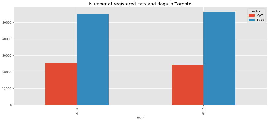
Let’s plot the total number of registered pets during each year.
df_sum_pets = df_animals.sum(axis=0).to_frame().T.drop(['FSA','TOTAL_2017','TOTAL_2013'],axis=1).T
df_sum_pets['Year'] = df_sum_pets.index.str[-4:]
df_sum_pets.columns=['Sum','Year']
df_sum_pets = df_sum_pets.reset_index()
df_sum_pets['index'] = df_sum_pets['index'].str[0:-5]
df_sum_pets = pd.pivot_table(df_sum_pets,values='Sum',index='Year',columns='index',aggfunc=np.sum)
df_sum_pets
| index | CAT | DOG |
|---|---|---|
| Year | ||
| 2013 | 25737 | 54864 |
| 2017 | 24489 | 56459 |
df_sum_pets.plot(kind='bar',
figsize=(15,6),
title='Number of registered cats and dogs in Toronto');
4.d Final Filtering
Before performing any analysis, we need to verify that each dataset contains the same set of postalcodes.
print("The animal registry data contains {} rows and {} columns.".format(df_animals.shape[0],df_animals.shape[1]))
The animal registry data contains 96 rows and 7 columns.
print("The census dataset contains {} rows and {} columns.".format(df_census_raw.shape[0],df_census_raw.shape[1]))
The census dataset contains 96 rows and 3 columns.
print("The postal dataset contains {} rows and {} columns.".format(df_toronto_postal.shape[0],df_toronto_postal.shape[1]))
The postal dataset contains 102 rows and 3 columns.
We display the ones that do not appear in all three sets.
df_toronto_postal[(~df_toronto_postal['PostalCode'].isin(df_animals['FSA']))]
| PostalCode | Borough | Neighborhood | |
|---|---|---|---|
| 60 | M5K | Downtown Toronto | Design Exchange, Toronto Dominion Centre |
| 61 | M5L | Downtown Toronto | Commerce Court, Victoria Hotel |
| 69 | M5W | Downtown Toronto | Stn A PO Boxes 25 The Esplanade |
| 70 | M5X | Downtown Toronto | First Canadian Place, Underground city |
| 85 | M7A | Queen's Park | Queen's Park |
| 87 | M7Y | East Toronto | Business Reply Mail Processing Centre 969 Eastern |
Note: These are neighborhoods that we have removed because they only contains fewer than 15 inhabitants. We remove these records from the Toronto postal data.
df_toronto_postal = df_toronto_postal[(df_toronto_postal['PostalCode'].isin(df_animals['FSA']))]
print('After cleaning:')
print("The postal dataset contains {} rows and {} columns.".format(df_toronto_postal.shape[0],df_toronto_postal.shape[1]))
After cleaning:
The postal dataset contains 96 rows and 3 columns.
We now have datasets that can be merged together. Before we do, we will add additional features. For instance, we want to add the latitude and longitude to the df_toronto_postal dataframe.
df_zip_toronto = pd.DataFrame(columns = list(df_toronto_postal.columns)+['Latitude','Longitude'])
print('Instantiate new dataframe:')
df_zip_toronto
Instantiate new dataframe:
| PostalCode | Borough | Neighborhood | Latitude | Longitude |
|---|
In order to geolocalize the neighborhood, we use the ARCGIS Service instead of the geocoder.google. ARCGIS is more reliable and gives accurate results after a single call to the API.
Geocoder Documentation: https://media.readthedocs.org/pdf/geocoder/latest/geocoder.pdf
# set counter of API calls
api_calls = 0
for postalcode, borough, neighborhood in zip(df_toronto_postal['PostalCode'],df_toronto_postal['Borough'],df_toronto_postal['Neighborhood']):
# initialize your variable to None
lat_lng_coords = None
# loop until you get the coordinates
while(lat_lng_coords is None):
g = geocoder.arcgis('{}, Toronto, Ontario,Canada'.format(postalcode))
lat_lng_coords = g.latlng
api_calls+=1
latitude = lat_lng_coords[0]
longitude = lat_lng_coords[1]
df_zip_toronto = df_zip_toronto.append({
'PostalCode':postalcode,
'Borough':borough,
'Neighborhood':neighborhood,
'Latitude':latitude,
'Longitude':longitude
},ignore_index=True)
print('All locations have been retrieved.')
print('{} calls to the API were made.'.format(api_calls))
All locations have been retrieved.
96 calls to the API were made.
print('New DataFrame populated with the latitude and longitude of each neighborhood:')
df_zip_toronto.head()
New DataFrame populated with the latitude and longitude of each neighborhood:
| PostalCode | Borough | Neighborhood | Latitude | Longitude | |
|---|---|---|---|---|---|
| 0 | M1B | Scarborough | Rouge, Malvern | 43.811650 | -79.195561 |
| 1 | M1C | Scarborough | Highland Creek, Rouge Hill, Port Union | 43.785605 | -79.158701 |
| 2 | M1E | Scarborough | Guildwood, Morningside, West Hill | 43.765690 | -79.175299 |
| 3 | M1G | Scarborough | Woburn | 43.768216 | -79.217610 |
| 4 | M1H | Scarborough | Cedarbrae | 43.769608 | -79.239440 |
print('Animal dataset:')
df_animals.head()
Animal dataset:
| FSA | CAT_2013 | DOG_2013 | TOTAL_2013 | CAT_2017 | DOG_2017 | TOTAL_2017 | |
|---|---|---|---|---|---|---|---|
| 0 | M1B | 293 | 674 | 967 | 285 | 627 | 912 |
| 1 | M1C | 387 | 967 | 1354 | 297 | 775 | 1072 |
| 2 | M1E | 536 | 1085 | 1621 | 467 | 963 | 1430 |
| 3 | M1G | 252 | 457 | 709 | 220 | 385 | 605 |
| 4 | M1H | 184 | 361 | 545 | 155 | 309 | 464 |
print('Census dataset:')
df_census_raw.head()
Census dataset:
| Geographic code | Population, 2016 | Private dwellings occupied by usual residents, 2016 | |
|---|---|---|---|
| 0 | M1B | 66108.0 | 20230.0 |
| 1 | M1C | 35626.0 | 11274.0 |
| 2 | M1E | 46943.0 | 17161.0 |
| 3 | M1G | 29690.0 | 9767.0 |
| 4 | M1H | 24383.0 | 8985.0 |
Note: Before we merge our datasets, we want to simplify the feature names by changing the name of the dataframe columns.
df_animals.columns = ['PostalCode','CatCount_2013','DogCount_2013','TotalPets_2013','CatCount_2017','DogCount_2017','TotalPets_2017']
df_census_raw.columns = ['PostalCode','Population2016','Dwellings2016']
print('Animal and Census dataset columns have been renamed...')
Animal and Census dataset columns have been renamed...
Note: We now merge the dataframe into one unique set.
df_merged = df_zip_toronto.merge(df_census_raw,on='PostalCode')
df_merged = df_merged.merge(df_animals,on='PostalCode')
print('All three datasets have been merged...')
All three datasets have been merged...
print("The merged dataset contains {} rows and {} columns.".format(df_merged.shape[0],df_merged.shape[1]))
The merged dataset contains 96 rows and 13 columns.
print('Merged dataset:')
df_merged.head()
Merged dataset:
| PostalCode | Borough | Neighborhood | Latitude | Longitude | Population2016 | Dwellings2016 | CatCount_2013 | DogCount_2013 | TotalPets_2013 | CatCount_2017 | DogCount_2017 | TotalPets_2017 | |
|---|---|---|---|---|---|---|---|---|---|---|---|---|---|
| 0 | M1B | Scarborough | Rouge, Malvern | 43.811650 | -79.195561 | 66108.0 | 20230.0 | 293 | 674 | 967 | 285 | 627 | 912 |
| 1 | M1C | Scarborough | Highland Creek, Rouge Hill, Port Union | 43.785605 | -79.158701 | 35626.0 | 11274.0 | 387 | 967 | 1354 | 297 | 775 | 1072 |
| 2 | M1E | Scarborough | Guildwood, Morningside, West Hill | 43.765690 | -79.175299 | 46943.0 | 17161.0 | 536 | 1085 | 1621 | 467 | 963 | 1430 |
| 3 | M1G | Scarborough | Woburn | 43.768216 | -79.217610 | 29690.0 | 9767.0 | 252 | 457 | 709 | 220 | 385 | 605 |
| 4 | M1H | Scarborough | Cedarbrae | 43.769608 | -79.239440 | 24383.0 | 8985.0 | 184 | 361 | 545 | 155 | 309 | 464 |
5. Existing Veterinarians
In this section, we use the Foursquare API to retrieve the location of veterinarians in the Toronto area. Note that the search is done using the latitude and longitude of each neighborhood, the distance used in the query is defined as 1500m. Even if it results in search results that do not belong to the neighborhood, it corresponds to a distance that customer will be willing to travel to visit a veterinary.
# @hidden_cell
# Connection to Foursquare API
CLIENT_ID = "BCHEH0XGR45MQ0DEPAW2Y1PAU3ETQUQC4Y2FXYXUKLZGAOBX"
CLIENT_SECRET = "KZJHNBUOPOXCG0CP3HBUDWJPV2DPBMTJHD33FKEVZ1YGL5UQ"
VERSION = '20180604'
print('Foursquare credentials have been defined....')
Foursquare credentials have been defined....
Let’s explore the first neighborhood in our dataframe.
Get the neighborhood’s latitude and longitude values.
neighborhood_latitude = df_merged.loc[1, 'Latitude'] # neighborhood latitude value
neighborhood_longitude = df_merged.loc[1, 'Longitude'] # neighborhood longitude value
neighborhood_name = df_merged.loc[1, 'Neighborhood'] # neighborhood name
print('Latitude and longitude values of {} are {}, {}.'.format(neighborhood_name,
neighborhood_latitude,
neighborhood_longitude))
Latitude and longitude values of Highland Creek, Rouge Hill, Port Union are 43.78560500000003, -79.15870110299994.
Now, let’s get the top veterinaries that are in Highland Creek, Rouge Hill, Port Union within a radius of 1500 meters.
# obtain top 100 venues in Rouge, Malvern wthin a radius of 1000 meters
radius = 2000
LIMIT = 50
VERSION = '20180604'
search_query = 'veterinarian'
url = 'https://api.foursquare.com/v2/venues/search?categoryId=4d954af4a243a5684765b473&client_id={}&client_secret={}&ll={},{}&v={}&radius={}&limit={}'.format(
CLIENT_ID,
CLIENT_SECRET,
neighborhood_latitude,
neighborhood_longitude,
VERSION,
radius,
LIMIT)
The following is the JSON file obtained from query to the Foursquare API.
results = requests.get(url).json()
results
{'meta': {'code': 200, 'requestId': '5c80438a1ed2196e4b561e51'},
'response': {'confident': True,
'venues': [{'categories': [{'icon': {'prefix': 'https://ss3.4sqi.net/img/categories_v2/building/medical_veterinarian_',
'suffix': '.png'},
'id': '4d954af4a243a5684765b473',
'name': 'Veterinarian',
'pluralName': 'Veterinarians',
'primary': True,
'shortName': 'Veterinarians'}],
'hasPerk': False,
'id': '4c8a28641797236a09de5e88',
'location': {'address': '5528 Lawrence Avenue East',
'cc': 'CA',
'city': 'Scarborough',
'country': 'Canada',
'distance': 1779,
'formattedAddress': ['5528 Lawrence Avenue East',
'Scarborough ON M1C 3B2',
'Canada'],
'labeledLatLngs': [{'label': 'display',
'lat': 43.779939844328915,
'lng': -79.13800246155462}],
'lat': 43.779939844328915,
'lng': -79.13800246155462,
'postalCode': 'M1C 3B2',
'state': 'ON'},
'name': 'West Hill Animal Clinic',
'referralId': 'v-1551909770'}]}}
print('The category of the venue is {}.'.format(results['response']['venues'][0]['categories'][0]['name']))
The category of the venue is Veterinarian.
# function that extracts the category of the venue
def get_category_type(row):
"""
Function:
Retrieve the category type from a venue.
Input:
Pandas DataFrame row.
Output:
Category name.
"""
try:
categories_list = row['categories']
except:
categories_list = row['venue.categories']
if len(categories_list) == 0:
return None
else:
return categories_list[0]['name']
def getNearbyVenues(postalcodes ,names, latitudes, longitudes, radius=3000):
"""
Function:
Use Foursquare API to retrieve the top 100 venues associated to a neighborhood.
Inputs:
names: pandas Series containing the names of the neighborhoods.
latitudes: pandas Series containing the latitudes of each neighborhood.
longitudes: pandas Series containing the longitudes of each neighborhood.
radius: maximum distance in meters between the center of the neighborhood and the venue.
Outputs:
pandas DataFrame containing the set of retrieved venues.
"""
# initiate an empty list of venues
venues_list=[]
index = 1
# loop through the data
for postal, name, lat, lng in zip(postalcodes, names, latitudes, longitudes):
# create the API request URL
url = 'https://api.foursquare.com/v2/venues/search?categoryId=4d954af4a243a5684765b473&client_id={}&client_secret={}&ll={},{}&v={}&radius={}&limit={}'.format(
CLIENT_ID,
CLIENT_SECRET,
lat,
lng,
VERSION,
radius,
LIMIT)
# make the GET request
results = requests.get(url).json()["response"]['venues']
# return only relevant information for each nearby venue
venues_list.append([(
postal,
name,
lat,
lng,
v['name'],
v['location']['lat'],
v['location']['lng'],
v['categories'][0]['name']) for v in results])
print('{}. {}: {} DONE...{} venues found.'.format(index,postal,name,len(results)))
index+=1
# create DataFrame from the list of venues
nearby_venues = pd.DataFrame([item for venue_list in venues_list for item in venue_list])
# set DataFrame columns
nearby_venues.columns = ['PostalCode',
'Neighborhood',
'Neighborhood Latitude',
'Neighborhood Longitude',
'Venue',
'Venue Latitude',
'Venue Longitude',
'Venue Category']
return(nearby_venues)
We run the query using the Foursquare API to retrieve the veterinarians for each neighborhood.
df_toronto_vets = getNearbyVenues(postalcodes=df_merged['PostalCode'],
names=df_merged['Neighborhood'],
latitudes=df_merged['Latitude'],
longitudes=df_merged['Longitude']
)
1. M1B: Rouge, Malvern DONE...1 venues found.
2. M1C: Highland Creek, Rouge Hill, Port Union DONE...1 venues found.
3. M1E: Guildwood, Morningside, West Hill DONE...1 venues found.
4. M1G: Woburn DONE...5 venues found.
5. M1H: Cedarbrae DONE...5 venues found.
6. M1J: Scarborough Village DONE...5 venues found.
7. M1K: East Birchmount Park, Ionview, Kennedy Park DONE...7 venues found.
8. M1L: Clairlea, Golden Mile, Oakridge DONE...8 venues found.
9. M1M: Cliffcrest, Cliffside, Scarborough Village West DONE...6 venues found.
10. M1N: Birch Cliff, Cliffside West DONE...8 venues found.
11. M1P: Dorset Park, Scarborough Town Centre, Wexford Heights DONE...10 venues found.
12. M1R: Maryvale, Wexford DONE...5 venues found.
13. M1S: Agincourt DONE...6 venues found.
14. M1T: Clarks Corners, Sullivan, Tam O'Shanter DONE...9 venues found.
15. M1V: Agincourt North, L'Amoreaux East, Milliken, Steeles East DONE...6 venues found.
16. M1W: L'Amoreaux West, Steeles West DONE...4 venues found.
17. M1X: Upper Rouge DONE...0 venues found.
18. M2H: Hillcrest Village DONE...1 venues found.
19. M2J: Fairview, Henry Farm, Oriole DONE...2 venues found.
20. M2K: Bayview Village DONE...7 venues found.
21. M2L: Silver Hills, York Mills DONE...10 venues found.
22. M2M: Newtonbrook, Willowdale DONE...9 venues found.
23. M2N: Willowdale South DONE...8 venues found.
24. M2P: York Mills West DONE...10 venues found.
25. M2R: Willowdale West DONE...5 venues found.
26. M3A: Parkwoods DONE...9 venues found.
27. M3B: Don Mills North DONE...8 venues found.
28. M3C: Flemingdon Park, Don Mills South DONE...4 venues found.
29. M3H: Bathurst Manor, Downsview North, Wilson Heights DONE...3 venues found.
30. M3J: Northwood Park, York University DONE...3 venues found.
31. M3K: CFB Toronto, Downsview East DONE...3 venues found.
32. M3L: Downsview West DONE...2 venues found.
33. M3M: Downsview Central DONE...3 venues found.
34. M3N: Downsview Northwest DONE...0 venues found.
35. M4A: Victoria Village DONE...5 venues found.
36. M4B: Woodbine Gardens, Parkview Hill DONE...4 venues found.
37. M4C: Woodbine Heights DONE...10 venues found.
38. M4E: The Beaches DONE...8 venues found.
39. M4G: Leaside DONE...7 venues found.
40. M4H: Thorncliffe Park DONE...10 venues found.
41. M4J: East Toronto DONE...16 venues found.
42. M4K: The Danforth West, Riverdale DONE...19 venues found.
43. M4L: The Beaches West, India Bazaar DONE...13 venues found.
44. M4M: Studio District DONE...14 venues found.
45. M4N: Lawrence Park DONE...11 venues found.
46. M4P: Davisville North DONE...8 venues found.
47. M4R: North Toronto West DONE...10 venues found.
48. M4S: Davisville DONE...12 venues found.
49. M4T: Moore Park, Summerhill East DONE...15 venues found.
50. M4V: Deer Park, Forest Hill SE, Rathnelly, South Hill, Summerhill West DONE...23 venues found.
51. M4W: Rosedale DONE...21 venues found.
52. M4X: Cabbagetown, St. James Town DONE...18 venues found.
53. M4Y: Church and Wellesley DONE...22 venues found.
54. M5A: Harbourfront, Regent Park DONE...19 venues found.
55. M5B: Ryerson, Garden District DONE...23 venues found.
56. M5C: St. James Town DONE...21 venues found.
57. M5E: Berczy Park DONE...15 venues found.
58. M5G: Central Bay Street DONE...24 venues found.
59. M5H: Adelaide, King, Richmond DONE...21 venues found.
60. M5J: Harbourfront East, Toronto Islands, Union Station DONE...6 venues found.
61. M5M: Bedford Park, Lawrence Manor East DONE...6 venues found.
62. M5N: Roselawn DONE...10 venues found.
63. M5P: Forest Hill North, Forest Hill West DONE...22 venues found.
64. M5R: The Annex, North Midtown, Yorkville DONE...26 venues found.
65. M5S: Harbord, University of Toronto DONE...28 venues found.
66. M5T: Chinatown, Grange Park, Kensington Market DONE...23 venues found.
67. M5V: CN Tower, Bathurst Quay, Island airport, Harbourfront West, King and Spadina, Railway Lands, South Niagara DONE...23 venues found.
68. M6A: Lawrence Heights, Lawrence Manor DONE...5 venues found.
69. M6B: Glencairn DONE...6 venues found.
70. M6C: Humewood-Cedarvale DONE...15 venues found.
71. M6E: Caledonia-Fairbanks DONE...9 venues found.
72. M6G: Christie DONE...27 venues found.
73. M6H: Dovercourt Village, Dufferin DONE...23 venues found.
74. M6J: Little Portugal, Trinity DONE...28 venues found.
75. M6K: Brockton, Exhibition Place, Parkdale Village DONE...21 venues found.
76. M6L: Maple Leaf Park, North Park, Upwood Park DONE...2 venues found.
77. M6M: Del Ray, Keelesdale, Mount Dennis, Silverthorn DONE...3 venues found.
78. M6N: The Junction North, Runnymede DONE...10 venues found.
79. M6P: High Park, The Junction South DONE...17 venues found.
80. M6R: Parkdale, Roncesvalles DONE...22 venues found.
81. M6S: Runnymede, Swansea DONE...16 venues found.
82. M8V: Humber Bay Shores, Mimico South, New Toronto DONE...1 venues found.
83. M8W: Alderwood, Long Branch DONE...4 venues found.
84. M8X: The Kingsway, Montgomery Road, Old Mill North DONE...12 venues found.
85. M8Y: Humber Bay, King's Mill Park, Kingsway Park South East, Mimico NE, Old Mill South, The Queensway East, Royal York South East, Sunnylea DONE...11 venues found.
86. M8Z: Kingsway Park South West, Mimico NW, The Queensway West, Royal York South West, South of Bloor DONE...7 venues found.
87. M9A: Islington Avenue DONE...11 venues found.
88. M9B: Cloverdale, Islington, Martin Grove, Princess Gardens, West Deane Park DONE...8 venues found.
89. M9C: Bloordale Gardens, Eringate, Markland Wood, Old Burnhamthorpe DONE...4 venues found.
90. M9L: Humber Summit DONE...2 venues found.
91. M9M: Emery, Humberlea DONE...2 venues found.
92. M9N: Weston DONE...2 venues found.
93. M9P: Westmount DONE...2 venues found.
94. M9R: Kingsview Village, Martin Grove Gardens, Richview Gardens, St. Phillips DONE...1 venues found.
95. M9V: Albion Gardens, Beaumond Heights, Humbergate, Jamestown, Mount Olive, Silverstone, South Steeles, Thistletown DONE...4 venues found.
96. M9W: Northwest DONE...3 venues found.
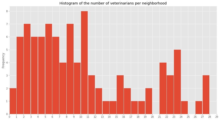
Let’s look at the distribution of veterinarians.
df_toronto_vets.head(1)
| PostalCode | Neighborhood | Neighborhood Latitude | Neighborhood Longitude | Venue | Venue Latitude | Venue Longitude | Venue Category | |
|---|---|---|---|---|---|---|---|---|
| 0 | M1B | Rouge, Malvern | 43.81165 | -79.195561 | Malvern Veterinary Hospital | 43.795586 | -79.226581 | Veterinarian |
df_toronto_vets_count = df_toronto_vets['PostalCode'].value_counts()
print("The grouped venue dataset contains {} rows.".format(df_toronto_vets_count.shape[0]))
The grouped venue dataset contains 94 rows.
Two neighborhood do not contain any venues, we identify them and add them manually in the venue count series.
df_merged[~df_merged['PostalCode'].isin(df_toronto_vets_count.index)]
| PostalCode | Borough | Neighborhood | Latitude | Longitude | Population2016 | Dwellings2016 | CatCount_2013 | DogCount_2013 | TotalPets_2013 | CatCount_2017 | DogCount_2017 | TotalPets_2017 | |
|---|---|---|---|---|---|---|---|---|---|---|---|---|---|
| 16 | M1X | Scarborough | Upper Rouge | 43.834215 | -79.216701 | 15097.0 | 3649.0 | 41 | 120 | 161 | 35 | 113 | 148 |
| 33 | M3N | North York | Downsview Northwest | 43.755356 | -79.519590 | 41958.0 | 13841.0 | 129 | 237 | 366 | 152 | 314 | 466 |
temp = pd.Series({'M1X':0,'M3N':0})
df_toronto_vets_count = df_toronto_vets_count.append(temp)
print('After modifications:')
print("The grouped venue dataset contains {} rows.".format(df_toronto_vets_count.shape[0]))
After modifications:
The grouped venue dataset contains 96 rows.
df_toronto_vets['Venue'].nunique()
129
df_toronto_vets_count.plot(kind='hist',
figsize=(15,8),
title='Histogram of the number of veterinarians per neighborhood',
rwidth=0.95,
bins=28,
xticks=list(range(0,30)),
xlim=(0,29));
6. Feature Engineering
In this section, we will combine the existing features to create new ones that are judged meaningfull for our study. The followings are added:
- Number of veterinarians per 1000 inhabitants
- Number of registered pets per 1000 inhabitants
- Number of registered cats per 1000 inhabitants
- Number of registered dogs per 1000 inhabitants
- Number of vets per 1000 registered pets
- Number of vets per 1000 registered inhabitants
- Number of registered pets per 1000 dwellings
- Number of vets per 1000 dwellings
- Proportion of cats
- Change in cat registration number
- Change in dog registration number
We first merge the dataframe containing the sum of venues to the main dataframe.
df_toronto_vets_count = df_toronto_vets_count.to_frame().reset_index()
df_toronto_vets_count.columns=['PostalCode','TotalVets']
df_toronto_vets_count.head()
| PostalCode | TotalVets | |
|---|---|---|
| 0 | M5S | 28 |
| 1 | M6J | 28 |
| 2 | M6G | 27 |
| 3 | M5R | 26 |
| 4 | M5G | 24 |
df_merged = df_merged.merge(df_toronto_vets_count, on='PostalCode')
df_merged_final = df_merged.copy()
FINAL DATASET
df_merged_final.head()
| PostalCode | Borough | Neighborhood | Latitude | Longitude | Population2016 | Dwellings2016 | CatCount_2013 | DogCount_2013 | TotalPets_2013 | CatCount_2017 | DogCount_2017 | TotalPets_2017 | TotalVets | |
|---|---|---|---|---|---|---|---|---|---|---|---|---|---|---|
| 0 | M1B | Scarborough | Rouge, Malvern | 43.811650 | -79.195561 | 66108.0 | 20230.0 | 293 | 674 | 967 | 285 | 627 | 912 | 1 |
| 1 | M1C | Scarborough | Highland Creek, Rouge Hill, Port Union | 43.785605 | -79.158701 | 35626.0 | 11274.0 | 387 | 967 | 1354 | 297 | 775 | 1072 | 1 |
| 2 | M1E | Scarborough | Guildwood, Morningside, West Hill | 43.765690 | -79.175299 | 46943.0 | 17161.0 | 536 | 1085 | 1621 | 467 | 963 | 1430 | 1 |
| 3 | M1G | Scarborough | Woburn | 43.768216 | -79.217610 | 29690.0 | 9767.0 | 252 | 457 | 709 | 220 | 385 | 605 | 5 |
| 4 | M1H | Scarborough | Cedarbrae | 43.769608 | -79.239440 | 24383.0 | 8985.0 | 184 | 361 | 545 | 155 | 309 | 464 | 5 |
Note: We create new features
df_merged_final['CatPerThousandInhab_2017'] = df_merged_final['CatCount_2017'] / df_merged_final['Population2016'] * 1000
df_merged_final['DogPerThousandInhab_2017'] = df_merged_final['DogCount_2017'] / df_merged_final['Population2016'] * 1000
df_merged_final['PetPerThousandInhab_2017'] = df_merged_final['TotalPets_2017'] / df_merged_final['Population2016'] * 1000
df_merged_final['VetPerPet_2017'] = df_merged_final['TotalVets'] / df_merged_final['TotalPets_2017']
df_merged_final['VetPerInhab'] = df_merged_final['TotalVets'] / df_merged_final['Population2016']
df_merged_final['PetPerThousandDwelling_2017'] = df_merged_final['TotalPets_2017'] / df_merged_final['Dwellings2016'] * 1000
df_merged_final['VetPerThousandDwelling'] = df_merged_final['TotalVets'] / df_merged_final['Dwellings2016'] * 1000
df_merged_final['PropCats_2017'] = df_merged_final['CatCount_2017'] / df_merged_final['TotalPets_2017'] * 100
df_merged_final['PropDogs_2017'] = df_merged_final['DogCount_2017'] / df_merged_final['TotalPets_2017'] * 100
df_merged_final['PropCats_2013'] = df_merged_final['CatCount_2013'] / df_merged_final['TotalPets_2013'] * 100
df_merged_final['PropDogs_2013'] = df_merged_final['DogCount_2013'] / df_merged_final['TotalPets_2013'] * 100
df_merged_final['DeltaCats'] = df_merged_final['CatCount_2017'] - df_merged_final['CatCount_2013']
df_merged_final['DeltaDogs'] = df_merged_final['DogCount_2017'] - df_merged_final['DogCount_2013']
df_merged_final['DeltaPets'] = df_merged_final['TotalPets_2017'] - df_merged_final['TotalPets_2013']
New features added to final dataset
df_merged_final.head()
| PostalCode | Borough | Neighborhood | Latitude | Longitude | Population2016 | Dwellings2016 | CatCount_2013 | DogCount_2013 | TotalPets_2013 | CatCount_2017 | DogCount_2017 | TotalPets_2017 | TotalVets | CatPerThousandInhab_2017 | DogPerThousandInhab_2017 | PetPerThousandInhab_2017 | VetPerPet_2017 | VetPerInhab | PetPerThousandDwelling_2017 | VetPerThousandDwelling | PropCats_2017 | PropDogs_2017 | PropCats_2013 | PropDogs_2013 | DeltaCats | DeltaDogs | DeltaPets | |
|---|---|---|---|---|---|---|---|---|---|---|---|---|---|---|---|---|---|---|---|---|---|---|---|---|---|---|---|---|
| 0 | M1B | Scarborough | Rouge, Malvern | 43.811650 | -79.195561 | 66108.0 | 20230.0 | 293 | 674 | 967 | 285 | 627 | 912 | 1 | 4.311127 | 9.484480 | 13.795607 | 0.001096 | 0.000015 | 45.081562 | 0.049432 | 31.250000 | 68.750000 | 30.299897 | 69.700103 | -8 | -47 | -55 |
| 1 | M1C | Scarborough | Highland Creek, Rouge Hill, Port Union | 43.785605 | -79.158701 | 35626.0 | 11274.0 | 387 | 967 | 1354 | 297 | 775 | 1072 | 1 | 8.336608 | 21.753775 | 30.090383 | 0.000933 | 0.000028 | 95.086039 | 0.088700 | 27.705224 | 72.294776 | 28.581979 | 71.418021 | -90 | -192 | -282 |
| 2 | M1E | Scarborough | Guildwood, Morningside, West Hill | 43.765690 | -79.175299 | 46943.0 | 17161.0 | 536 | 1085 | 1621 | 467 | 963 | 1430 | 1 | 9.948235 | 20.514241 | 30.462476 | 0.000699 | 0.000021 | 83.328477 | 0.058272 | 32.657343 | 67.342657 | 33.066009 | 66.933991 | -69 | -122 | -191 |
| 3 | M1G | Scarborough | Woburn | 43.768216 | -79.217610 | 29690.0 | 9767.0 | 252 | 457 | 709 | 220 | 385 | 605 | 5 | 7.409902 | 12.967329 | 20.377231 | 0.008264 | 0.000168 | 61.943278 | 0.511928 | 36.363636 | 63.636364 | 35.543018 | 64.456982 | -32 | -72 | -104 |
| 4 | M1H | Scarborough | Cedarbrae | 43.769608 | -79.239440 | 24383.0 | 8985.0 | 184 | 361 | 545 | 155 | 309 | 464 | 5 | 6.356888 | 12.672764 | 19.029652 | 0.010776 | 0.000205 | 51.641625 | 0.556483 | 33.405172 | 66.594828 | 33.761468 | 66.238532 | -29 | -52 | -81 |
7. Exploration and Analysis
In this section we will create several map plots. In order to understand feature distribution across the various neighborhoods, visualization tools are used.
# url to be scrapped
URL_geojson = 'https://raw.githubusercontent.com/ag2816/Visualizations/master/data/Toronto2.geojson'
# GET request
request = requests.get(URL_geojson)
data = request.text
print('GEOJSON file loaded...')
GEOJSON file loaded...
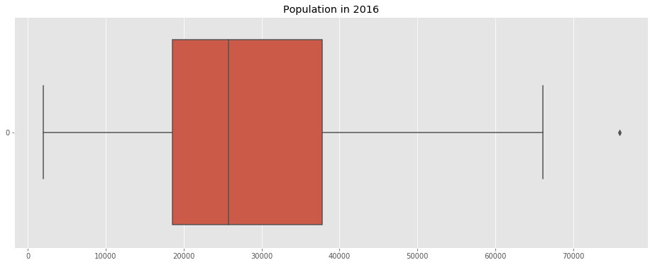
7.a. Population Distribution
Using Folium, we plot the population distribution in the Toronto area:
LATITUDE, LONGITUDE = [43.722898, -79.381049]
print('The latitude and longitude of Toronto are {}, {}'.format(LATITUDE,LONGITUDE))
The latitude and longitude of Toronto are 43.722898, -79.381049
f, ax = plt.subplots(figsize=(16,6))
ax.set_title('Population in 2016')
sns.boxplot(data=df_merged_final['Population2016'],ax=ax,orient='h');
state_geo = data
m = folium.Map(location=[LATITUDE,LONGITUDE], zoom_start=11)
folium.Choropleth(
geo_data=state_geo,
name='choropleth',
data=df_merged_final,
columns=['PostalCode', 'Population2016'],
key_on='feature.properties.CFSAUID',
fill_color='YlOrRd',
fill_opacity=0.7,
line_opacity=0.2,
legend_name='Total Population'
).add_to(m)
folium.LayerControl().add_to(m)
m
7.b. Animal Distribution
print('Neighborhoods with largest pet ratio (pet per thousand people:)')
df_merged_final[['PostalCode','Borough','Neighborhood','PetPerThousandInhab_2017']].sort_values(by='PetPerThousandInhab_2017',ascending=False).head(3)
Neighborhoods with largest pet ratio (pet per thousand people:)
| PostalCode | Borough | Neighborhood | PetPerThousandInhab_2017 | |
|---|---|---|---|---|
| 37 | M4E | East Toronto | The Beaches | 64.326785 |
| 79 | M6R | West Toronto | Parkdale, Roncesvalles | 60.281009 |
| 82 | M8W | Etobicoke | Alderwood, Long Branch | 58.769469 |
print('Neighborhoods with smallest pet ratio (pet per thousand people:)')
df_merged_final[['PostalCode','Borough','Neighborhood','PetPerThousandInhab_2017']].sort_values(by='PetPerThousandInhab_2017',ascending=True).head(3)
Neighborhoods with smallest pet ratio (pet per thousand people:)
| PostalCode | Borough | Neighborhood | PetPerThousandInhab_2017 | |
|---|---|---|---|---|
| 39 | M4H | East York | Thorncliffe Park | 6.399837 |
| 16 | M1X | Scarborough | Upper Rouge | 9.803272 |
| 33 | M3N | North York | Downsview Northwest | 11.106344 |
Notes:
- Above are listed with three neighborhoods with the highest and lowest number of pets per thousand people.
- The highest ownership rate is 64 pets for one thousand people in “The Beaches”.
- The lowest ownership rate is 6 pets for one thousand people in “Thorncliffe Park”.
state_geo = data
m = folium.Map(location=[LATITUDE,LONGITUDE], zoom_start=11)
folium.Choropleth(
geo_data=state_geo,
name='choropleth',
data=df_merged_final,
columns=['PostalCode', 'PetPerThousandInhab_2017'],
key_on='feature.properties.CFSAUID',
fill_color='RdBu',
fill_opacity=0.8,
line_opacity=0.2,
legend_name='Number of pets per one thousand inhabitants'
).add_to(m)
folium.LayerControl().add_to(m)
m
7.c. Change in Animal Registration
state_geo = data
m = folium.Map(location=[LATITUDE,LONGITUDE], zoom_start=11)
folium.Choropleth(
geo_data=state_geo,
name='choropleth',
data=df_merged_final,
columns=['PostalCode', 'DeltaPets'],
key_on='feature.properties.CFSAUID',
fill_color='RdYlGn',
fill_opacity=0.8,
line_opacity=0.2,
legend_name='Change in number of registered animals between 2013 and 2017'
).add_to(m)
folium.LayerControl().add_to(m)
m
From the above map, we can see that on average, neighborhoods tend to have the same number of pets. However, there are a few extreme cases.
f, ax = plt.subplots(figsize=(16,6))
ax.set_title('Boxplot of change in registered pet between 2013 and 2017')
sns.boxplot(data=df_merged_final[['DeltaCats','DeltaDogs','DeltaPets']],ax=ax,orient='h');
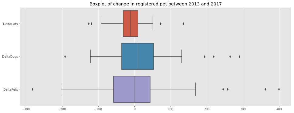
The following observations can be made from the above plot:
- On average, the number of cats per neighborhood seems to decrease.
- On average, the number of dogs per neighborhood seems to decrease.
state_geo = data
m = folium.Map(location=[LATITUDE,LONGITUDE], zoom_start=11)
folium.Choropleth(
geo_data=state_geo,
name='choropleth',
data=df_merged_final,
columns=['PostalCode', 'DeltaCats'],
key_on='feature.properties.CFSAUID',
fill_color='RdYlGn',
fill_opacity=0.8,
line_opacity=0.2,
legend_name='Change in number of registered cats between 2013 and 2017'
).add_to(m)
folium.LayerControl().add_to(m)
m
state_geo = data
m = folium.Map(location=[LATITUDE,LONGITUDE], zoom_start=11)
folium.Choropleth(
geo_data=state_geo,
name='choropleth',
data=df_merged_final,
columns=['PostalCode', 'DeltaDogs'],
key_on='feature.properties.CFSAUID',
fill_color='RdYlGn',
fill_opacity=0.8,
line_opacity=0.2,
legend_name='Change in number of registered dogs between 2013 and 2017'
).add_to(m)
folium.LayerControl().add_to(m)
m
7.d. Vet distribution
In this section, we will look at the distribution of vet in the city. Let’s start by looking at the neighborhoods with the highest and lowest veterinarians per people.
df_merged_final[['PostalCode','Borough','Neighborhood','VetPerInhab']].sort_values(by='VetPerInhab',ascending=True).head(3)
| PostalCode | Borough | Neighborhood | VetPerInhab | |
|---|---|---|---|---|
| 33 | M3N | North York | Downsview Northwest | 0.000000 |
| 16 | M1X | Scarborough | Upper Rouge | 0.000000 |
| 0 | M1B | Scarborough | Rouge, Malvern | 0.000015 |
df_merged_final[['PostalCode','Borough','Neighborhood','VetPerInhab']].sort_values(by='VetPerInhab',ascending=False).head(3)
| PostalCode | Borough | Neighborhood | VetPerInhab | |
|---|---|---|---|---|
| 58 | M5H | Downtown Toronto | Adelaide, King, Richmond | 0.010474 |
| 55 | M5C | Downtown Toronto | St. James Town | 0.007116 |
| 57 | M5G | Downtown Toronto | Central Bay Street | 0.002849 |
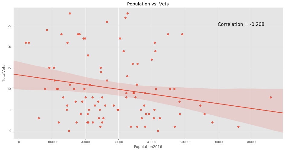
We plot the data to get a better understanding of the distribution of vets throughout the city.
f, ax = plt.subplots(figsize=(16,8))
ax.set_title('Population vs. Vets')
p = sns.regplot(x='Population2016',y='TotalVets',data=df_merged_final,ax=ax);
p.text(60000,25,
'Correlation = {:.3f}'.format(np.corrcoef(df_merged_final['Population2016'],df_merged_final['TotalVets'])[0,1]),
fontsize=15);
f, ax = plt.subplots(figsize=(16,6))
ax.set_title('Boxplot vet per inhabitant')
sns.boxplot(data=df_merged_final[['VetPerInhab']],ax=ax,orient='h');
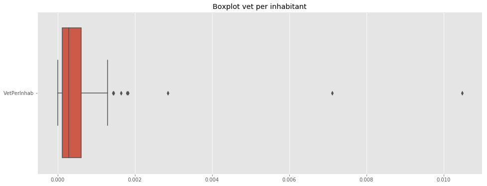
Note: The above distribution shows a uneven distribution in the proportion of vets per neighborhood.
state_geo = data
m = folium.Map(location=[LATITUDE,LONGITUDE], zoom_start=11)
folium.Choropleth(
geo_data=state_geo,
name='choropleth',
data=df_merged_final,
columns=['PostalCode', 'TotalVets'],
key_on='feature.properties.CFSAUID',
fill_color='Accent',
fill_opacity=0.8,
line_opacity=0.2,
legend_name='Number of vets in the proximity of the neighborhood'
).add_to(m)
folium.LayerControl().add_to(m)
m
df_temp = df_merged_final[['PostalCode', 'VetPerPet_2017']].copy()
df_temp['HasVets'] = df_temp['VetPerPet_2017'].copy()
df_temp.loc[df_temp['VetPerPet_2017']==0,'HasVets'] = np.nan
df_temp['HasVetsLog'] = np.log10(df_temp['HasVets'])
state_geo = data
m = folium.Map(location=[LATITUDE,LONGITUDE], zoom_start=11)
folium.Choropleth(
geo_data=state_geo,
name='choropleth',
data=df_temp,
columns=['PostalCode', 'HasVetsLog'],
key_on='feature.properties.CFSAUID',
fill_color='RdYlGn',
fill_opacity=0.8,
line_opacity=0.2,
legend_name='Number of Vets per pets - Log Scale'
).add_to(m)
folium.LayerControl().add_to(m)
m
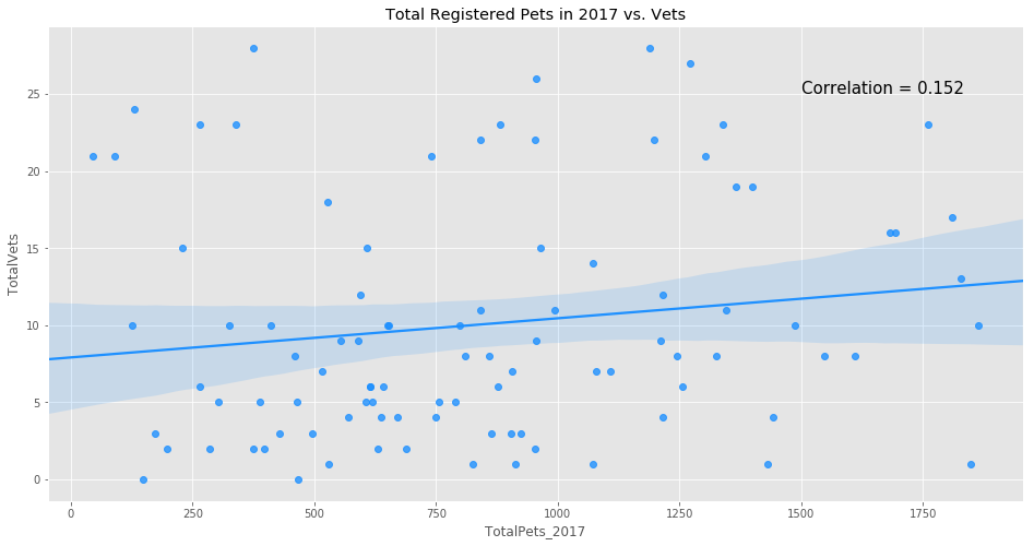
We now look at the distribution of vets against the pet distribution.
Below are the neighborhoods with the highest and lowest vet to pet ratio.
df_merged_final[['PostalCode','Borough','Neighborhood','VetPerPet_2017']].sort_values(by='VetPerPet_2017',ascending=True).head(3)
| PostalCode | Borough | Neighborhood | VetPerPet_2017 | |
|---|---|---|---|---|
| 33 | M3N | North York | Downsview Northwest | 0.000000 |
| 16 | M1X | Scarborough | Upper Rouge | 0.000000 |
| 81 | M8V | Etobicoke | Humber Bay Shores, Mimico South, New Toronto | 0.000541 |
df_merged_final[['PostalCode','Borough','Neighborhood','VetPerPet_2017']].sort_values(by='VetPerPet_2017',ascending=False).head(3)
| PostalCode | Borough | Neighborhood | VetPerPet_2017 | |
|---|---|---|---|---|
| 58 | M5H | Downtown Toronto | Adelaide, King, Richmond | 0.477273 |
| 55 | M5C | Downtown Toronto | St. James Town | 0.230769 |
| 57 | M5G | Downtown Toronto | Central Bay Street | 0.183206 |
f, ax = plt.subplots(figsize=(16,8))
ax.set_title('Total Registered Pets in 2017 vs. Vets')
p = sns.regplot(x='TotalPets_2017',y='TotalVets',data=df_merged_final,ax=ax,color='dodgerblue');
p.text(1500,25,
'Correlation = {:.3f}'.format(np.corrcoef(df_merged_final['TotalPets_2017'],df_merged_final['TotalVets'])[0,1]),
fontsize=15);
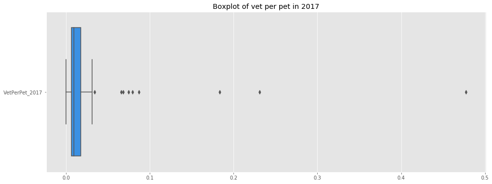
f, ax = plt.subplots(figsize=(16,6))
ax.set_title('Boxplot of vet per pet in 2017')
sns.boxplot(data=df_merged_final[['VetPerPet_2017']],ax=ax,orient='h',color='dodgerblue');
7.e. Cat vs Dog Friendly Neighborhoods
In this section we will investigate the distribution of cats and dogs in Toronto.
First, we look at the neighborhoods where the dogs represent more than 70% of the registered cats and dogs in 2017.
# very dog-friendly neighborhoods
df_merged_final[['PostalCode','Borough','Neighborhood','PropDogs_2017']][df_merged_final['PropDogs_2017']>70].sort_values(by='PropDogs_2017',ascending=False)
| PostalCode | Borough | Neighborhood | PropDogs_2017 | |
|---|---|---|---|---|
| 58 | M5H | Downtown Toronto | Adelaide, King, Richmond | 86.363636 |
| 44 | M4N | Central Toronto | Lawrence Park | 84.185493 |
| 50 | M4W | Downtown Toronto | Rosedale | 82.432432 |
| 48 | M4T | Central Toronto | Moore Park, Summerhill East | 81.219110 |
| 61 | M5N | Central Toronto | Roselawn | 81.010720 |
| 49 | M4V | Central Toronto | Deer Park, Forest Hill SE, Rathnelly, South Hi... | 80.272109 |
| 60 | M5M | North York | Bedford Park, Lawrence Manor East | 79.920319 |
| 23 | M2P | North York | York Mills West | 79.692308 |
| 62 | M5P | Central Toronto | Forest Hill North, Forest Hill West | 79.664570 |
| 55 | M5C | Downtown Toronto | St. James Town | 78.021978 |
| 20 | M2L | North York | Silver Hills, York Mills | 77.804878 |
| 56 | M5E | Downtown Toronto | Berczy Park | 76.419214 |
| 16 | M1X | Scarborough | Upper Rouge | 76.351351 |
| 26 | M3B | North York | Don Mills North | 76.252723 |
| 68 | M6B | North York | Glencairn | 76.168224 |
| 31 | M3L | North York | Downsview West | 75.874126 |
| 69 | M6C | York | Humewood-Cedarvale | 75.207469 |
| 63 | M5R | Central Toronto | The Annex, North Midtown, Yorkville | 74.345550 |
| 38 | M4G | East York | Leaside | 74.328082 |
| 83 | M8X | Etobicoke | The Kingsway, Montgomery Road, Old Mill North | 74.242424 |
| 11 | M1R | Scarborough | Maryvale, Wexford | 74.039735 |
| 46 | M4R | Central Toronto | North Toronto West | 73.886329 |
| 47 | M4S | Central Toronto | Davisville | 73.848684 |
| 66 | M5V | Downtown Toronto | CN Tower, Bathurst Quay, Island airport, Harbo... | 73.656716 |
| 89 | M9L | North York | Humber Summit | 73.604061 |
| 43 | M4M | East Toronto | Studio District | 73.507463 |
| 37 | M4E | East Toronto | The Beaches | 73.308504 |
| 19 | M2K | North York | Bayview Village | 73.307544 |
| 86 | M9A | Etobicoke | Islington Avenue | 73.254086 |
| 28 | M3H | North York | Bathurst Manor, Downsview North, Wilson Heights | 73.051948 |
| 1 | M1C | Scarborough | Highland Creek, Rouge Hill, Port Union | 72.294776 |
| 42 | M4L | East Toronto | The Beaches West, India Bazaar | 71.936543 |
| 76 | M6M | York | Del Ray, Keelesdale, Mount Dennis, Silverthorn | 71.842410 |
| 52 | M4Y | Downtown Toronto | Church and Wellesley | 71.819263 |
| 91 | M9N | York | Weston | 71.802326 |
| 65 | M5T | Downtown Toronto | Chinatown, Grange Park, Kensington Market | 71.597633 |
| 8 | M1M | Scarborough | Cliffcrest, Cliffside, Scarborough Village West | 71.493729 |
| 45 | M4P | Central Toronto | Davisville North | 71.478463 |
| 84 | M8Y | Etobicoke | Humber Bay, King's Mill Park, Kingsway Park So... | 71.227364 |
| 95 | M9W | Etobicoke | Northwest | 70.764120 |
| 70 | M6E | York | Caledonia-Fairbanks | 70.544554 |
| 30 | M3K | North York | CFB Toronto, Downsview East | 70.520231 |
| 14 | M1V | Scarborough | Agincourt North, L'Amoreaux East, Milliken, St... | 70.406504 |
| 59 | M5J | Downtown Toronto | Harbourfront East, Toronto Islands, Union Station | 70.188679 |
| 88 | M9C | Etobicoke | Bloordale Gardens, Eringate, Markland Wood, Ol... | 70.110957 |
# extremely dog-friendly neighborhoods
df_merged_final[['PostalCode','Borough','Neighborhood','PropDogs_2017']][df_merged_final['PropDogs_2017']>80].sort_values(by='PropDogs_2017',ascending=False)
| PostalCode | Borough | Neighborhood | PropDogs_2017 | |
|---|---|---|---|---|
| 58 | M5H | Downtown Toronto | Adelaide, King, Richmond | 86.363636 |
| 44 | M4N | Central Toronto | Lawrence Park | 84.185493 |
| 50 | M4W | Downtown Toronto | Rosedale | 82.432432 |
| 48 | M4T | Central Toronto | Moore Park, Summerhill East | 81.219110 |
| 61 | M5N | Central Toronto | Roselawn | 81.010720 |
| 49 | M4V | Central Toronto | Deer Park, Forest Hill SE, Rathnelly, South Hi... | 80.272109 |
Notes:
- Adelaide, King, Richmond are the neighborhoods with the highest dog proportion (86.36%)
- Thorncliffe Park is the neighborhood with the lowest dog proportion (54.76%)
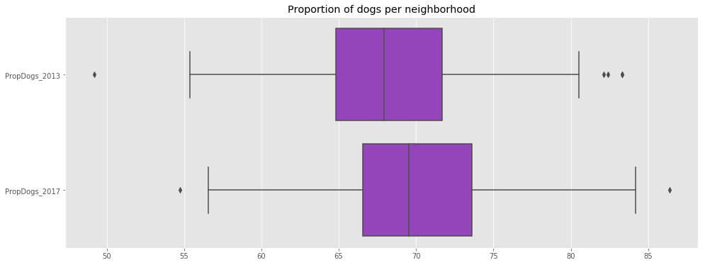
f, ax = plt.subplots(figsize=(16,6))
ax.set_title('Proportion of dogs per neighborhood')
sns.boxplot(data=df_merged_final[['PropDogs_2013','PropDogs_2017']],ax=ax,orient='h',color='darkorchid');
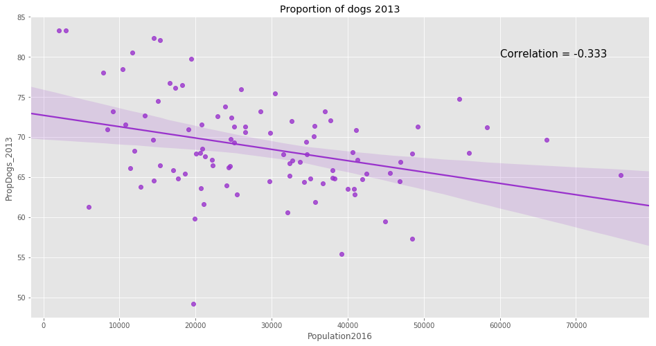
f, ax = plt.subplots(figsize=(16,8))
ax.set_title('Proportion of dogs 2013')
p = sns.regplot(x='Population2016',y='PropDogs_2013',data=df_merged_final,ax=ax,color='darkorchid');
p.text(60000,80,
'Correlation = {:.3f}'.format(np.corrcoef(df_merged_final['Population2016'],df_merged_final['PropDogs_2013'])[0,1]),
fontsize=15);
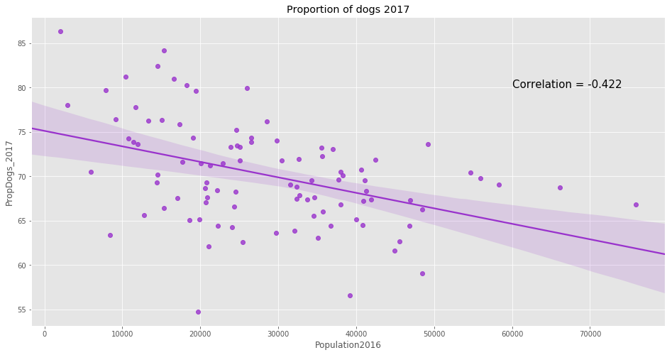
f, ax = plt.subplots(figsize=(16,8))
ax.set_title('Proportion of dogs 2017')
p = sns.regplot(x='Population2016',y='PropDogs_2017',data=df_merged_final,ax=ax,color='darkorchid');
p.text(60000,80,
'Correlation = {:.3f}'.format(np.corrcoef(df_merged_final['Population2016'],df_merged_final['PropDogs_2017'])[0,1]),
fontsize=15);
As shown above, there is no neighborhood in 2017 where there are more registered cats than there are registered dogs. In addition, it appears that the proportion of dogs has increased between 2013 and 2017.
Moreover, the data shows that the more populated the neighborhood, the lesser is the proportion of dogs. This can be explained as dogs require more space and people tend to have dogs once they live in houses in neighborhood with a lesser population density.
state_geo = data
m = folium.Map(location=[LATITUDE,LONGITUDE], zoom_start=11)
folium.Choropleth(
geo_data=state_geo,
name='choropleth',
data=df_merged_final,
columns=['PostalCode', 'PropDogs_2013'],
key_on='feature.properties.CFSAUID',
fill_color='BuPu',
fill_opacity=0.8,
line_opacity=0.2,
legend_name='Proportion of dogs in 2013'
).add_to(m)
folium.LayerControl().add_to(m)
m
state_geo = data
m = folium.Map(location=[LATITUDE,LONGITUDE], zoom_start=11)
folium.Choropleth(
geo_data=state_geo,
name='choropleth',
data=df_merged_final,
columns=['PostalCode', 'PropDogs_2017'],
key_on='feature.properties.CFSAUID',
fill_color='BuPu',
fill_opacity=0.8,
line_opacity=0.2,
legend_name='Proportion of dogs in 2017'
).add_to(m)
folium.LayerControl().add_to(m)
m
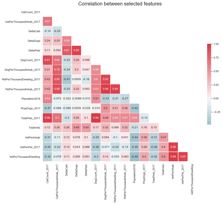
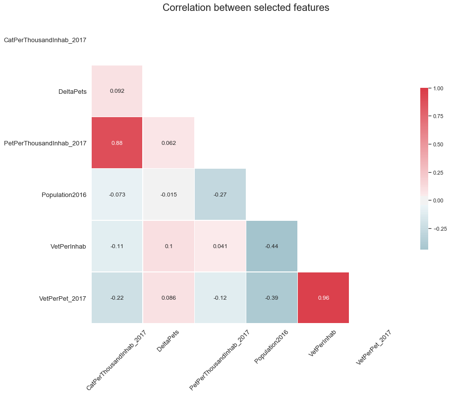
7.f. Feature correlations
sns.set(style="white")
# Compute the correlation matrix
omitted_columns = ['Latitude','Longitude','CatCount_2013','DogCount_2013',
'TotalPets_2013','PropCats_2013','PropDogs_2013','PropCats_2017',
'Borough','Dwellings2016','PostalCode']
df_temp = df_merged_final[df_merged_final.columns.difference(omitted_columns)]
corr = df_temp.corr()
# Generate a mask for the upper triangle
mask = np.zeros_like(corr, dtype=np.bool)
mask[np.triu_indices_from(mask)] = True
# Set up the matplotlib figure
f, ax = plt.subplots(figsize=(14, 12))
ax.set_title('Correlation between selected features',fontsize=20)
# Generate a custom diverging colormap
cmap = sns.diverging_palette(220, 10, as_cmap=True)
# Draw the heatmap with the mask and correct aspect ratio
sns.heatmap(corr, mask=mask, cmap=cmap, vmax=1.00, center=0,
square=True, linewidths=.5, cbar_kws={"shrink": .5},
annot=True,);
8. Clustering
Now that we have a good understanding of the pet and vet distribution in the city, we leverage the power of clustering to find out which neighborhoods are the best candidate for a new veterinarian.
print('Features not included in model:\n')
omitted_columns = ['Latitude','Longitude','CatCount_2013','DogCount_2013',
'TotalPets_2013','PropCats_2013','PropDogs_2013','PropCats_2017',
'Borough','Dwellings2016','PostalCode','Neighborhood',
'CatCount_2017','DogCount_2017','TotalPets_2017','TotalVets',
'DeltaDogs','DeltaCats','PropDogs_2017','PetPerThousandDwelling_2017','VetPerThousandDwelling',
'DogPerThousandInhab_2017']
selected_columns = df_merged_final.columns.difference(omitted_columns)
print(omitted_columns)
print('\nFeatures included in model:\n')
print(selected_columns)
Features not included in model:
['Latitude', 'Longitude', 'CatCount_2013', 'DogCount_2013', 'TotalPets_2013', 'PropCats_2013', 'PropDogs_2013', 'PropCats_2017', 'Borough', 'Dwellings2016', 'PostalCode', 'Neighborhood', 'CatCount_2017', 'DogCount_2017', 'TotalPets_2017', 'TotalVets', 'DeltaDogs', 'DeltaCats', 'PropDogs_2017', 'PetPerThousandDwelling_2017', 'VetPerThousandDwelling', 'DogPerThousandInhab_2017']
Features included in model:
Index(['CatPerThousandInhab_2017', 'DeltaPets', 'PetPerThousandInhab_2017', 'Population2016', 'VetPerInhab', 'VetPerPet_2017'], dtype='object')
Now that the data has been filtered, we copy in into a training set.
X_train = df_merged_final[selected_columns].copy()
print('Training set ready...')
Training set ready...
sns.set_style("ticks", {"xtick.major.size": 40, "ytick.major.size": 8})
sns.set(style="white")
# Compute the correlation matrix
omitted_columns = ['Latitude','Longitude','CatCount_2013','DogCount_2013',
'TotalPets_2013','PropCats_2013','PropDogs_2013','PropCats_2017',
'Borough','Dwellings2016','PostalCode']
df_temp = df_merged_final[df_merged_final.columns.difference(omitted_columns)]
corr = X_train.corr()
# Generate a mask for the upper triangle
mask = np.zeros_like(corr, dtype=np.bool)
mask[np.triu_indices_from(mask)] = True
# Set up the matplotlib figure
f, ax = plt.subplots(figsize=(14, 12))
ax.set_title('Correlation between selected features',fontsize=20)
ax.tick_params(axis='both', which='major', labelsize=13)
# Generate a custom diverging colormap
cmap = sns.diverging_palette(220, 10, as_cmap=True)
# Draw the heatmap with the mask and correct aspect ratio
g = sns.heatmap(corr, mask=mask, cmap=cmap, vmax=1.00, center=0,
square=True, linewidths=.5, cbar_kws={"shrink": .5},
annot=True,)
g.set_xticklabels(g.get_xticklabels(), rotation = 45, fontsize = 13);
print('Scaling data using standard scaler...')
scaler = StandardScaler()
X_train = scaler.fit_transform(X_train)
X_train = pd.DataFrame(X_train, index=df_merged_final.index, columns=selected_columns)
X_train.head()
print('Data is scaled.')
Scaling data using standard scaler...
Data is scaled.
In order to group similar neighborhoods, we use a K-means clustering algorithm. We iterate over the number of clusterss in order to find the best value for this hyperparameter.
# define candidates to n_clusters
num_clusters = range(1, 96)
# instantiate the K-means algorithm
kmeans = [KMeans(n_clusters=i,n_init=20,random_state=100) for i in num_clusters]
# store scores
score = [kmeans[i].fit(X_train).score(X_train) for i in range(len(kmeans))]
# compute first derivative of elbow curve
score_prime = np.array(score)
score_prime = np.diff(score_prime,n=1) / score_prime[0:-1]
# reset plotting style
plt.style.use('ggplot')
# best n_cluster value
best_param = 9
# create plot
f, axes = plt.subplots(nrows=1, ncols=2,figsize=(16, 6))
# elbow curve
axes[0].plot(num_clusters, score)
axes[0].set_xlabel('Number of Clusters')
axes[0].set_ylabel('Score')
axes[0].set_title('Elbow Curve')
axes[0].set_xticks(list(range(0,96,5)))
axes[0].plot([best_param,best_param],[min(score),max(score)],linestyle='dashed')
# first derivative
axes[1].plot(num_clusters[0:-1],score_prime)
axes[1].set_xlabel('Number of Clusters')
axes[1].set_ylabel('First derivative of score')
axes[1].set_title('First derivative of elbow curve')
axes[1].set_xticks(list(range(0,96,5)))
axes[1].plot([best_param,best_param],[min(score_prime),max(score_prime)],linestyle='dashed');
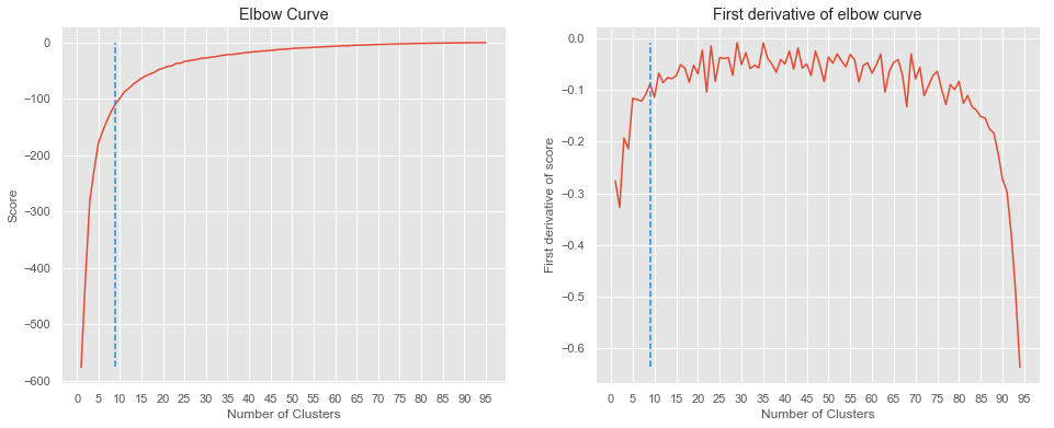
From the above plot, it appears that the best number of cluster (using the elbow method) is n_cluster=9.
# set number of clusters
kclusters = 9
# run k-means clustering
kmeans = KMeans(n_clusters=kclusters, n_init=20,random_state=100).fit(X_train)
# check cluster labels generated for each row in the dataframe
kmeans.labels_[0:5]
array([5, 0, 0, 4, 4], dtype=int32)
print('Cluster distribution:')
np.array(np.unique(kmeans.labels_, return_counts=True)).T
Cluster distribution:
array([[ 0, 10],
[ 1, 15],
[ 2, 1],
[ 3, 9],
[ 4, 24],
[ 5, 14],
[ 6, 17],
[ 7, 1],
[ 8, 5]])
We now insert the results of the clustering to our original dataframe.
df_merged_final['Cluster'] = kmeans.labels_
print('Overview of the clustering:\n')
df_merged_final.head()
Overview of the clustering:
| PostalCode | Borough | Neighborhood | Latitude | Longitude | Population2016 | Dwellings2016 | CatCount_2013 | DogCount_2013 | TotalPets_2013 | CatCount_2017 | DogCount_2017 | TotalPets_2017 | TotalVets | CatPerThousandInhab_2017 | DogPerThousandInhab_2017 | PetPerThousandInhab_2017 | VetPerPet_2017 | VetPerInhab | PetPerThousandDwelling_2017 | VetPerThousandDwelling | PropCats_2017 | PropDogs_2017 | PropCats_2013 | PropDogs_2013 | DeltaCats | DeltaDogs | DeltaPets | Cluster | |
|---|---|---|---|---|---|---|---|---|---|---|---|---|---|---|---|---|---|---|---|---|---|---|---|---|---|---|---|---|---|
| 0 | M1B | Scarborough | Rouge, Malvern | 43.811650 | -79.195561 | 66108.0 | 20230.0 | 293 | 674 | 967 | 285 | 627 | 912 | 1 | 4.311127 | 9.484480 | 13.795607 | 0.001096 | 0.000015 | 45.081562 | 0.049432 | 31.250000 | 68.750000 | 30.299897 | 69.700103 | -8 | -47 | -55 | 5 |
| 1 | M1C | Scarborough | Highland Creek, Rouge Hill, Port Union | 43.785605 | -79.158701 | 35626.0 | 11274.0 | 387 | 967 | 1354 | 297 | 775 | 1072 | 1 | 8.336608 | 21.753775 | 30.090383 | 0.000933 | 0.000028 | 95.086039 | 0.088700 | 27.705224 | 72.294776 | 28.581979 | 71.418021 | -90 | -192 | -282 | 0 |
| 2 | M1E | Scarborough | Guildwood, Morningside, West Hill | 43.765690 | -79.175299 | 46943.0 | 17161.0 | 536 | 1085 | 1621 | 467 | 963 | 1430 | 1 | 9.948235 | 20.514241 | 30.462476 | 0.000699 | 0.000021 | 83.328477 | 0.058272 | 32.657343 | 67.342657 | 33.066009 | 66.933991 | -69 | -122 | -191 | 0 |
| 3 | M1G | Scarborough | Woburn | 43.768216 | -79.217610 | 29690.0 | 9767.0 | 252 | 457 | 709 | 220 | 385 | 605 | 5 | 7.409902 | 12.967329 | 20.377231 | 0.008264 | 0.000168 | 61.943278 | 0.511928 | 36.363636 | 63.636364 | 35.543018 | 64.456982 | -32 | -72 | -104 | 4 |
| 4 | M1H | Scarborough | Cedarbrae | 43.769608 | -79.239440 | 24383.0 | 8985.0 | 184 | 361 | 545 | 155 | 309 | 464 | 5 | 6.356888 | 12.672764 | 19.029652 | 0.010776 | 0.000205 | 51.641625 | 0.556483 | 33.405172 | 66.594828 | 33.761468 | 66.238532 | -29 | -52 | -81 | 4 |
We create a map to visualize the different clusters.
step = folium.StepColormap(['red','lime','cyan',
'darkorchid','royalblue','pink','gold',
'limegreen','orange','gray'],vmin=0.0, vmax=9)
print('colormap used for to differentiate clusters:')
step
colormap used for to differentiate clusters:
m = folium.Map(location=[LATITUDE,LONGITUDE], zoom_start=11)
folium.GeoJson(
state_geo,
style_function=lambda feature: {
'fillColor': step(df_merged_final.set_index('PostalCode')['Cluster'][feature['properties']['CFSAUID']]),
'color' : 'black',
'weight' : 0.5,
'fillOpacity':0.6
}
).add_to(m)
# set color scheme for the clusters
colors_array = step
rainbow = ['red','lime','cyan',
'darkorchid','royalblue','pink','gold',
'limegreen','orange','gray']
# add markers to the map
markers_colors = []
for lat, lon, poi, cluster in zip(df_merged_final['Latitude'], df_merged_final['Longitude'], df_merged_final['Neighborhood'], df_merged_final['Cluster']):
label = folium.Popup(str(poi) + ' Cluster ' + str(cluster), parse_html=True)
folium.CircleMarker(
[lat, lon],
radius=2,
popup=label,
color='k',
fill=True,
fill_color='k',
fill_opacity=1.0).add_to(m)
folium.LayerControl().add_to(m)
m
Let’s now print the average features per cluster.
df_cluster_grouped = df_merged_final.groupby('Cluster').mean()
df_cluster_grouped = df_cluster_grouped.reset_index()
df_cluster_grouped
| Cluster | Latitude | Longitude | Population2016 | Dwellings2016 | CatCount_2013 | DogCount_2013 | TotalPets_2013 | CatCount_2017 | DogCount_2017 | TotalPets_2017 | TotalVets | CatPerThousandInhab_2017 | DogPerThousandInhab_2017 | PetPerThousandInhab_2017 | VetPerPet_2017 | VetPerInhab | PetPerThousandDwelling_2017 | VetPerThousandDwelling | PropCats_2017 | PropDogs_2017 | PropCats_2013 | PropDogs_2013 | DeltaCats | DeltaDogs | DeltaPets | |
|---|---|---|---|---|---|---|---|---|---|---|---|---|---|---|---|---|---|---|---|---|---|---|---|---|---|---|
| 0 | 0 | 43.703557 | -79.426277 | 39269.900000 | 14928.900000 | 464.700000 | 960.600000 | 1425.300000 | 397.200000 | 903.400000 | 1300.600000 | 6.000000 | 10.056994 | 23.123213 | 33.180207 | 0.004470 | 0.000156 | 87.135669 | 0.396126 | 30.102639 | 69.897361 | 32.263283 | 67.736717 | -67.500000 | -57.200000 | -124.700000 |
| 1 | 1 | 43.668249 | -79.403617 | 23485.266667 | 9999.333333 | 411.533333 | 811.066667 | 1222.600000 | 371.600000 | 836.066667 | 1207.666667 | 12.266667 | 15.893231 | 36.428972 | 52.322204 | 0.010676 | 0.000549 | 123.328286 | 1.286108 | 30.617851 | 69.382149 | 33.599542 | 66.400458 | -39.933333 | 25.000000 | -14.933333 |
| 2 | 2 | 43.651210 | -79.375481 | 2951.000000 | 1721.000000 | 13.000000 | 65.000000 | 78.000000 | 20.000000 | 71.000000 | 91.000000 | 21.000000 | 6.777364 | 24.059641 | 30.837004 | 0.230769 | 0.007116 | 52.876235 | 12.202208 | 21.978022 | 78.021978 | 16.666667 | 83.333333 | 7.000000 | 6.000000 | 13.000000 |
| 3 | 3 | 43.649773 | -79.413452 | 38003.888889 | 19819.888889 | 391.333333 | 772.000000 | 1163.333333 | 446.444444 | 945.555556 | 1392.000000 | 18.666667 | 11.734882 | 25.232417 | 36.967299 | 0.014774 | 0.000506 | 74.031677 | 0.996972 | 31.419474 | 68.580526 | 32.443513 | 67.556487 | 55.111111 | 173.555556 | 228.666667 |
| 4 | 4 | 43.739205 | -79.396245 | 24314.708333 | 9132.583333 | 160.375000 | 337.833333 | 498.208333 | 157.166667 | 337.291667 | 494.458333 | 5.208333 | 6.197776 | 13.501303 | 19.699079 | 0.012978 | 0.000221 | 52.508247 | 0.557808 | 31.813534 | 68.186466 | 32.649561 | 67.350439 | -3.208333 | -0.541667 | -3.750000 |
| 5 | 5 | 43.763928 | -79.354505 | 49444.142857 | 17544.214286 | 281.000000 | 545.214286 | 826.214286 | 269.500000 | 527.571429 | 797.071429 | 4.642857 | 5.493784 | 10.633927 | 16.127711 | 0.005995 | 0.000098 | 45.361538 | 0.276678 | 33.770711 | 66.229289 | 33.922932 | 66.077068 | -11.500000 | -17.642857 | -29.142857 |
| 6 | 6 | 43.713203 | -79.399228 | 17700.470588 | 7860.705882 | 190.764706 | 565.176471 | 755.941176 | 172.882353 | 580.058824 | 752.941176 | 12.235294 | 9.525350 | 32.883828 | 42.409178 | 0.017489 | 0.000756 | 98.221346 | 1.710462 | 23.119539 | 76.880461 | 25.568207 | 74.431793 | -17.882353 | 14.882353 | -3.000000 |
| 7 | 7 | 43.649700 | -79.382582 | 2005.000000 | 1243.000000 | 5.000000 | 25.000000 | 30.000000 | 6.000000 | 38.000000 | 44.000000 | 21.000000 | 2.992519 | 18.952618 | 21.945137 | 0.477273 | 0.010474 | 35.398230 | 16.894610 | 13.636364 | 86.363636 | 16.666667 | 83.333333 | 1.000000 | 13.000000 | 14.000000 |
| 8 | 8 | 43.655050 | -79.387163 | 12689.200000 | 6816.800000 | 70.200000 | 141.000000 | 211.200000 | 83.000000 | 184.600000 | 267.600000 | 22.600000 | 6.468906 | 14.498019 | 20.966926 | 0.095643 | 0.001882 | 38.323887 | 3.403225 | 31.312799 | 68.687201 | 32.157574 | 67.842426 | 12.800000 | 43.600000 | 56.400000 |
colors = ['red','lime','cyan',
'darkorchid','royalblue','pink','gold',
'limegreen','orange','gray']
plt.style.use('ggplot')
f, ax = plt.subplots(figsize=(16,16))
for g in np.unique(df_merged_final['Cluster']):
ax.scatter(x = df_merged_final['PetPerThousandInhab_2017'][df_merged_final['Cluster']==g],
y = df_merged_final['VetPerPet_2017'][df_merged_final['Cluster']==g],
marker = 'o',
linewidth = 0,
s = df_merged_final['Population2016'][df_merged_final['Cluster']==g]/40,
c = colors[g],
label = 'Cluster ' + str(g),
alpha = 0.6
)
ax.set_xlabel('Pet Per Thousand Inhabitants 2017')
ax.set_ylabel('Veterinarians Per Pet 2017')
ax.set_yscale("log")
ax.set_ylim([10**-4,10**0])
ax.set_title('Clusters distributions based on pet/inhab and vet/pet')
legend = ax.legend(frameon=True,title='Size: Population')
for legend_handle in legend.legendHandles:
legend_handle._sizes = [50]
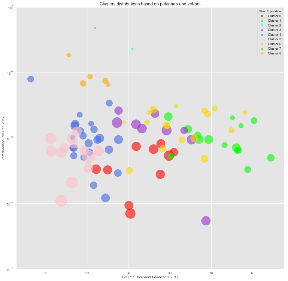
Note:
From the above, it appears that red, blue, and purple clusters present the best characteristics. They have few veterinarians per pets and a large number of pets per inhabitants.
colors = ['red','lime','cyan',
'darkorchid','royalblue','pink','gold',
'limegreen','orange','gray']
plt.style.use('ggplot')
f, ax = plt.subplots(figsize=(16,16))
for g in np.unique(df_merged_final['Cluster']):
ax.scatter(x = df_merged_final['DeltaPets'][df_merged_final['Cluster']==g],
y = df_merged_final['VetPerPet_2017'][df_merged_final['Cluster']==g],
marker = 'o',
linewidth = 0,
s = df_merged_final['PetPerThousandInhab_2017'][df_merged_final['Cluster']==g]*20,
c = colors[g],
label = 'Cluster ' + str(g),
alpha = 0.6
)
ax.set_xlabel('Change in number of registered pets')
ax.set_ylabel('Veterinarian per pet')
ax.set_yscale("log")
ax.set_ylim([10**-4,10**0])
ax.set_title('Clusters distributions based on population and number of pets')
legend = ax.legend(frameon=True,title='Size: Pet per inhab.')
for legend_handle in legend.legendHandles:
legend_handle._sizes = [50]
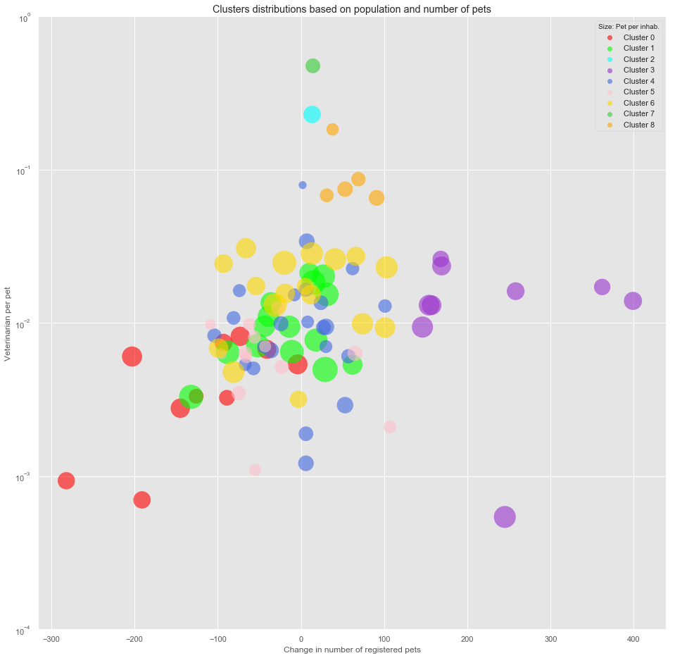
From the above plots, Cluster 3 is selected. As oppose to the other candidate (Cluster 0), the number of registered pets in the neighborhoods of Cluster 3 has increased between 2013 and 2017.
df_merged_final[df_merged_final['Cluster']==3]
| PostalCode | Borough | Neighborhood | Latitude | Longitude | Population2016 | Dwellings2016 | CatCount_2013 | DogCount_2013 | TotalPets_2013 | CatCount_2017 | DogCount_2017 | TotalPets_2017 | TotalVets | CatPerThousandInhab_2017 | DogPerThousandInhab_2017 | PetPerThousandInhab_2017 | VetPerPet_2017 | VetPerInhab | PetPerThousandDwelling_2017 | VetPerThousandDwelling | PropCats_2017 | PropDogs_2017 | PropCats_2013 | PropDogs_2013 | DeltaCats | DeltaDogs | DeltaPets | Cluster | |
|---|---|---|---|---|---|---|---|---|---|---|---|---|---|---|---|---|---|---|---|---|---|---|---|---|---|---|---|---|---|
| 43 | M4M | East Toronto | Studio District | 43.662766 | -79.334830 | 24689.0 | 10787.0 | 253 | 665 | 918 | 284 | 788 | 1072 | 14 | 11.503099 | 31.917048 | 43.420147 | 0.013060 | 0.000567 | 99.378882 | 1.297859 | 26.492537 | 73.507463 | 27.559913 | 72.440087 | 31 | 123 | 154 | 3 |
| 52 | M4Y | Downtown Toronto | Church and Wellesley | 43.666585 | -79.381302 | 30472.0 | 19665.0 | 165 | 508 | 673 | 237 | 604 | 841 | 22 | 7.777632 | 19.821475 | 27.599107 | 0.026159 | 0.000722 | 42.766336 | 1.118739 | 28.180737 | 71.819263 | 24.517088 | 75.482912 | 72 | 96 | 168 | 3 |
| 53 | M5A | Downtown Toronto | Harbourfront, Regent Park | 43.655120 | -79.362640 | 41078.0 | 22333.0 | 281 | 685 | 966 | 416 | 949 | 1365 | 19 | 10.127075 | 23.102391 | 33.229466 | 0.013919 | 0.000463 | 61.120315 | 0.850759 | 30.476190 | 69.523810 | 29.089027 | 70.910973 | 135 | 264 | 399 | 3 |
| 66 | M5V | Downtown Toronto | CN Tower, Bathurst Quay, Island airport, Harbo... | 43.640815 | -79.399538 | 49195.0 | 30726.0 | 281 | 697 | 978 | 353 | 987 | 1340 | 23 | 7.175526 | 20.063015 | 27.238541 | 0.017164 | 0.000468 | 43.611274 | 0.748552 | 26.343284 | 73.656716 | 28.732106 | 71.267894 | 72 | 290 | 362 | 3 |
| 72 | M6H | West Toronto | Dovercourt Village, Dufferin | 43.665087 | -79.438705 | 44950.0 | 19209.0 | 650 | 954 | 1604 | 676 | 1085 | 1761 | 23 | 15.038932 | 24.137931 | 39.176863 | 0.013061 | 0.000512 | 91.675777 | 1.197355 | 38.387280 | 61.612720 | 40.523691 | 59.476309 | 26 | 131 | 157 | 3 |
| 73 | M6J | West Toronto | Little Portugal, Trinity | 43.648525 | -79.417757 | 32684.0 | 15063.0 | 336 | 684 | 1020 | 382 | 807 | 1189 | 28 | 11.687676 | 24.690980 | 36.378656 | 0.023549 | 0.000857 | 78.935139 | 1.858859 | 32.127839 | 67.872161 | 32.941176 | 67.058824 | 46 | 123 | 169 | 3 |
| 74 | M6K | West Toronto | Brockton, Exhibition Place, Parkdale Village | 43.639410 | -79.425436 | 40957.0 | 22023.0 | 388 | 657 | 1045 | 427 | 876 | 1303 | 21 | 10.425568 | 21.388285 | 31.813854 | 0.016117 | 0.000513 | 59.165418 | 0.953549 | 32.770530 | 67.229470 | 37.129187 | 62.870813 | 39 | 219 | 258 | 3 |
| 78 | M6P | West Toronto | High Park, The Junction South | 43.659730 | -79.462812 | 40035.0 | 18972.0 | 606 | 1057 | 1663 | 630 | 1179 | 1809 | 17 | 15.736231 | 29.449232 | 45.185463 | 0.009397 | 0.000425 | 95.351044 | 0.896057 | 34.825871 | 65.174129 | 36.440168 | 63.559832 | 24 | 122 | 146 | 3 |
| 81 | M8V | Etobicoke | Humber Bay Shores, Mimico South, New Toronto | 43.609920 | -79.498049 | 37975.0 | 19601.0 | 562 | 1041 | 1603 | 613 | 1235 | 1848 | 1 | 16.142199 | 32.521396 | 48.663594 | 0.000541 | 0.000026 | 94.280904 | 0.051018 | 33.170996 | 66.829004 | 35.059264 | 64.940736 | 51 | 194 | 245 | 3 |
step = folium.StepColormap(['gray','purple'],vmin=0.0, vmax=1.0)
m = folium.Map(location=[LATITUDE,LONGITUDE], zoom_start=11)
folium.GeoJson(
state_geo,
style_function=lambda feature: {
'fillColor': step(df_merged_final.set_index('PostalCode')['Cluster'][feature['properties']['CFSAUID']]==3),
'color' : 'black',
'weight' : 0.5,
'fillOpacity':0.6
}
).add_to(m)
folium.LayerControl().add_to(m)
m
We now look at the trend in the number of registered animal for the cluster 3.
df_cluster_selected = df_merged_final[(df_merged_final['Cluster']==3)]
df_cluster_selected
| PostalCode | Borough | Neighborhood | Latitude | Longitude | Population2016 | Dwellings2016 | CatCount_2013 | DogCount_2013 | TotalPets_2013 | CatCount_2017 | DogCount_2017 | TotalPets_2017 | TotalVets | CatPerThousandInhab_2017 | DogPerThousandInhab_2017 | PetPerThousandInhab_2017 | VetPerPet_2017 | VetPerInhab | PetPerThousandDwelling_2017 | VetPerThousandDwelling | PropCats_2017 | PropDogs_2017 | PropCats_2013 | PropDogs_2013 | DeltaCats | DeltaDogs | DeltaPets | Cluster | |
|---|---|---|---|---|---|---|---|---|---|---|---|---|---|---|---|---|---|---|---|---|---|---|---|---|---|---|---|---|---|
| 43 | M4M | East Toronto | Studio District | 43.662766 | -79.334830 | 24689.0 | 10787.0 | 253 | 665 | 918 | 284 | 788 | 1072 | 14 | 11.503099 | 31.917048 | 43.420147 | 0.013060 | 0.000567 | 99.378882 | 1.297859 | 26.492537 | 73.507463 | 27.559913 | 72.440087 | 31 | 123 | 154 | 3 |
| 52 | M4Y | Downtown Toronto | Church and Wellesley | 43.666585 | -79.381302 | 30472.0 | 19665.0 | 165 | 508 | 673 | 237 | 604 | 841 | 22 | 7.777632 | 19.821475 | 27.599107 | 0.026159 | 0.000722 | 42.766336 | 1.118739 | 28.180737 | 71.819263 | 24.517088 | 75.482912 | 72 | 96 | 168 | 3 |
| 53 | M5A | Downtown Toronto | Harbourfront, Regent Park | 43.655120 | -79.362640 | 41078.0 | 22333.0 | 281 | 685 | 966 | 416 | 949 | 1365 | 19 | 10.127075 | 23.102391 | 33.229466 | 0.013919 | 0.000463 | 61.120315 | 0.850759 | 30.476190 | 69.523810 | 29.089027 | 70.910973 | 135 | 264 | 399 | 3 |
| 66 | M5V | Downtown Toronto | CN Tower, Bathurst Quay, Island airport, Harbo... | 43.640815 | -79.399538 | 49195.0 | 30726.0 | 281 | 697 | 978 | 353 | 987 | 1340 | 23 | 7.175526 | 20.063015 | 27.238541 | 0.017164 | 0.000468 | 43.611274 | 0.748552 | 26.343284 | 73.656716 | 28.732106 | 71.267894 | 72 | 290 | 362 | 3 |
| 72 | M6H | West Toronto | Dovercourt Village, Dufferin | 43.665087 | -79.438705 | 44950.0 | 19209.0 | 650 | 954 | 1604 | 676 | 1085 | 1761 | 23 | 15.038932 | 24.137931 | 39.176863 | 0.013061 | 0.000512 | 91.675777 | 1.197355 | 38.387280 | 61.612720 | 40.523691 | 59.476309 | 26 | 131 | 157 | 3 |
| 73 | M6J | West Toronto | Little Portugal, Trinity | 43.648525 | -79.417757 | 32684.0 | 15063.0 | 336 | 684 | 1020 | 382 | 807 | 1189 | 28 | 11.687676 | 24.690980 | 36.378656 | 0.023549 | 0.000857 | 78.935139 | 1.858859 | 32.127839 | 67.872161 | 32.941176 | 67.058824 | 46 | 123 | 169 | 3 |
| 74 | M6K | West Toronto | Brockton, Exhibition Place, Parkdale Village | 43.639410 | -79.425436 | 40957.0 | 22023.0 | 388 | 657 | 1045 | 427 | 876 | 1303 | 21 | 10.425568 | 21.388285 | 31.813854 | 0.016117 | 0.000513 | 59.165418 | 0.953549 | 32.770530 | 67.229470 | 37.129187 | 62.870813 | 39 | 219 | 258 | 3 |
| 78 | M6P | West Toronto | High Park, The Junction South | 43.659730 | -79.462812 | 40035.0 | 18972.0 | 606 | 1057 | 1663 | 630 | 1179 | 1809 | 17 | 15.736231 | 29.449232 | 45.185463 | 0.009397 | 0.000425 | 95.351044 | 0.896057 | 34.825871 | 65.174129 | 36.440168 | 63.559832 | 24 | 122 | 146 | 3 |
| 81 | M8V | Etobicoke | Humber Bay Shores, Mimico South, New Toronto | 43.609920 | -79.498049 | 37975.0 | 19601.0 | 562 | 1041 | 1603 | 613 | 1235 | 1848 | 1 | 16.142199 | 32.521396 | 48.663594 | 0.000541 | 0.000026 | 94.280904 | 0.051018 | 33.170996 | 66.829004 | 35.059264 | 64.940736 | 51 | 194 | 245 | 3 |
df_cluster_selected[['TotalPets_2013','TotalPets_2017']].set_index(df_cluster_selected['PostalCode']).T
| PostalCode | M4M | M4Y | M5A | M5V | M6H | M6J | M6K | M6P | M8V |
|---|---|---|---|---|---|---|---|---|---|
| TotalPets_2013 | 918 | 673 | 966 | 978 | 1604 | 1020 | 1045 | 1663 | 1603 |
| TotalPets_2017 | 1072 | 841 | 1365 | 1340 | 1761 | 1189 | 1303 | 1809 | 1848 |
plt.style.use('ggplot')
f, ax = plt.subplots(figsize=(8,10))
df_cluster_selected[['TotalPets_2013','TotalPets_2017']].set_index(df_cluster_selected['PostalCode']).T.plot(ax=ax)
ax.set_title('Change in number of registered pets for the neighborhoods of cluster 3')
ax.set_xlabel('Year')
ax.set_ylabel('Number of registered pets');
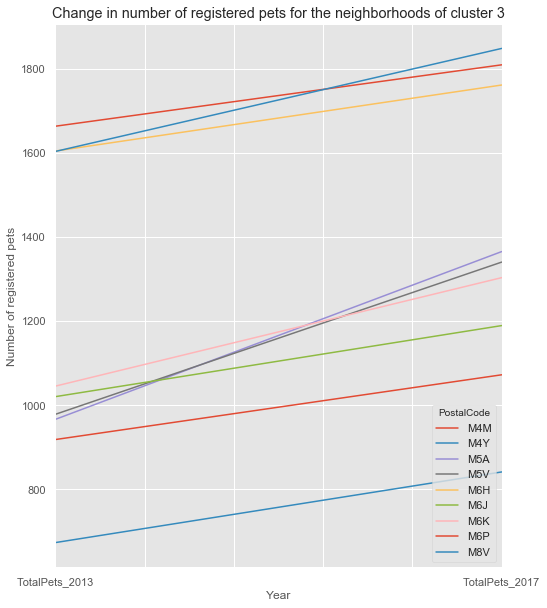
We refine the selection of the cluster 4 to the 5 neighborhoods with the highest vet to pet ratio
df_cluster_selected.set_index(df_cluster_selected['PostalCode'])['VetPerPet_2017'].sort_values(ascending=False)
PostalCode
M4Y 0.026159
M6J 0.023549
M5V 0.017164
M6K 0.016117
M5A 0.013919
M6H 0.013061
M4M 0.013060
M6P 0.009397
M8V 0.000541
Name: VetPerPet_2017, dtype: float64
df_cluster_selected_fil = df_cluster_selected.set_index(df_cluster_selected['PostalCode']).sort_values(by=['VetPerPet_2017'],ascending=False).head(5)
We mow inspect the variation in registered pets for thes 5 candidates.
df_cluster_selected_fil['DeltaPets'].sort_values(ascending=False)
PostalCode
M5A 399
M5V 362
M6K 258
M6J 169
M4Y 168
Name: DeltaPets, dtype: int64
CONCLUSION:
With the available data, it seems that the neighborhood M5A, M5V, and M6K represent the best opportunities for a new veterinarian.
best_neigh = df_cluster_selected.loc[df_cluster_selected['PostalCode'].isin(['M5A','M5V','M6K']),:].sort_values(by='DeltaPets',ascending=False)
best_neigh
| PostalCode | Borough | Neighborhood | Latitude | Longitude | Population2016 | Dwellings2016 | CatCount_2013 | DogCount_2013 | TotalPets_2013 | CatCount_2017 | DogCount_2017 | TotalPets_2017 | TotalVets | CatPerThousandInhab_2017 | DogPerThousandInhab_2017 | PetPerThousandInhab_2017 | VetPerPet_2017 | VetPerInhab | PetPerThousandDwelling_2017 | VetPerThousandDwelling | PropCats_2017 | PropDogs_2017 | PropCats_2013 | PropDogs_2013 | DeltaCats | DeltaDogs | DeltaPets | Cluster | |
|---|---|---|---|---|---|---|---|---|---|---|---|---|---|---|---|---|---|---|---|---|---|---|---|---|---|---|---|---|---|
| 53 | M5A | Downtown Toronto | Harbourfront, Regent Park | 43.655120 | -79.362640 | 41078.0 | 22333.0 | 281 | 685 | 966 | 416 | 949 | 1365 | 19 | 10.127075 | 23.102391 | 33.229466 | 0.013919 | 0.000463 | 61.120315 | 0.850759 | 30.476190 | 69.523810 | 29.089027 | 70.910973 | 135 | 264 | 399 | 3 |
| 66 | M5V | Downtown Toronto | CN Tower, Bathurst Quay, Island airport, Harbo... | 43.640815 | -79.399538 | 49195.0 | 30726.0 | 281 | 697 | 978 | 353 | 987 | 1340 | 23 | 7.175526 | 20.063015 | 27.238541 | 0.017164 | 0.000468 | 43.611274 | 0.748552 | 26.343284 | 73.656716 | 28.732106 | 71.267894 | 72 | 290 | 362 | 3 |
| 74 | M6K | West Toronto | Brockton, Exhibition Place, Parkdale Village | 43.639410 | -79.425436 | 40957.0 | 22023.0 | 388 | 657 | 1045 | 427 | 876 | 1303 | 21 | 10.425568 | 21.388285 | 31.813854 | 0.016117 | 0.000513 | 59.165418 | 0.953549 | 32.770530 | 67.229470 | 37.129187 | 62.870813 | 39 | 219 | 258 | 3 |
rank = ['gold','silver','#a87900']
size = [5, 5, 5]
m = folium.Map(location=[LATITUDE,LONGITUDE], zoom_start=11)
folium.GeoJson(
state_geo,
style_function=lambda feature: {
'fillColor': step(feature['properties']['CFSAUID'] in ['M5A','M5V','M6K']),
'color' : 'black',
'weight' : 0.5,
'fillOpacity':0.6
}
).add_to(m)
index=0
for lat, lon, poi in zip(best_neigh['Latitude'], best_neigh['Longitude'], best_neigh['Neighborhood']):
label = folium.Popup(str(poi) + '\nOption: ' + str(index+1), parse_html=True)
folium.CircleMarker(
[lat, lon],
radius=size[index],
popup=label,
color=rank[index],
fill=True,
fill_color=rank[index],
fill_opacity=1.0).add_to(m)
index+=1
folium.LayerControl().add_to(m)
m