Introduction
The purpose of this notebook is to dive deeper into backward pass of neural network models. In the first part of this series, we explored the concept of Generative AI and built a simple model that generates text using a bigram model and a single-layer neural network (NN). In the second part, we built a more complex model using a Multi-Layer Perceptron (MLP) to generate text, and in the third part, we explored the initialization of neural network models.
Table of Contents
- Data Loading and Cleanup
- Data Cleaning
- Model Parameters and Training Data
- Model Architecture
- Manual Backward Pass
- Validation of Manual Backward Pass
- Backward Pass Optimization
- Model Training
Data loading and cleanup
import torch
import torch.nn.functional as F
import matplotlib.pyplot as plt
import random
%matplotlib inline
# Define the path to our bird names dataset
DATASET_PATH = "./datasets/birds/birds.csv"

# Load the dataset: read the CSV file and split into lines (one bird name per line)
birds = open(DATASET_PATH, "r").read().splitlines()

# Display the first 10 bird names to get a sense of the data
print("First 10 birds in the dataset:\n")
print(", ".join(birds[:10]))
print(f"There are {len(birds):,d} birds in the dataset.")

min_length = map(len, birds)
max_length = map(len, birds)
print(f"\nThe shortest character name has {min(min_length)} characters.")
print(f"The longest character name has {max(max_length)} characters.")
First 10 birds in the dataset:

Abbott's babbler, Abbott's booby, Abbott's starling, Abbott's sunbird, Abd al-Kuri sparrow, Abdim's stork, Aberdare cisticola, Aberrant bush warbler, Abert's towhee, Abyssinian catbird
There are 10,976 birds in the dataset.

The shortest character name has 3 characters.
The longest character name has 35 characters.
Data Cleaning
Before we can use the bird names for training our neural network, we need to clean and standardize the data. Raw text data often contains inconsistencies that can make training more difficult, so we’ll apply several preprocessing steps to ensure our dataset is uniform and ready for tokenization.
The cleaning process we’ll implement includes:
- Whitespace normalization: Removing leading and trailing spaces
- Case standardization: Converting all text to lowercase for consistency
- Character filtering: Removing accents and special characters that might complicate tokenization
- Space handling: Replacing spaces with underscores to create valid single tokens
- Tokenization mapping: Creating bidirectional mappings between characters and numerical indices
This preprocessing step is crucial for ensuring our model receives clean, consistent input data that will lead to better training results.
from unidecode import unidecode

def clean_name(name):
    """
    Clean the bird name by applying several preprocessing steps:
    - Removing leading and trailing whitespaces
    - Converting to lowercase for consistency
    - Removing accents and special characters
    - Replacing spaces with underscores to create valid single tokens

    This function ensures all bird names are standardized for consistent tokenization.
    """
    # Remove leading/trailing spaces and convert to lowercase
    name = name.strip().lower()

    # Replace special characters with spaces, keeping only alphanumeric and space characters
    # This helps remove punctuation, symbols, and other non-standard characters
    name = ''.join(char if char.isalnum() or char.isspace() else ' ' for char in name)

    # Handle specific cases: replace apostrophes and spaces with underscores
    name = name.replace("`", "_")  # Remove apostrophes (common in bird names like "Abbott's")
    name = name.replace(" ", "_")  # Replace spaces with underscores for tokenization

    # Remove any remaining accents using unidecode (e.g., "café" becomes "cafe")
    name = unidecode(name)

    return name
# Apply the cleaning function to all bird names in the dataset
# This standardizes all names for consistent processing
birds = list(map(clean_name, birds))

# Create a vocabulary mapping for character-level tokenization
# Extract all unique characters from all bird names
unique_tokens = set([c for w in birds for c in w])

# Define a special token to mark the end of each bird name
# This helps the model learn when a name ends
SPECIAL_TOKEN = "."

# Create bidirectional mappings between characters and numerical indices
# index_to_token: maps index (0, 1, 2, ...) to character ('a', 'b', 'c', ...)
# token_to_index: maps character ('a', 'b', 'c', ...) to index (0, 1, 2, ...)
index_to_token = {i: t for i, t in enumerate(unique_tokens, start=1)}
token_to_index = {v: k for k, v in index_to_token.items()}

# Reserve index 0 for the special token (end-of-name marker)
index_to_token[0] = SPECIAL_TOKEN
token_to_index[SPECIAL_TOKEN] = 0

# Calculate vocabulary size (number of unique tokens + special token)
vocab_size = len(unique_tokens) + 1

# Display tokenization information for verification
print(f"Number of unique tokens: {len(unique_tokens)}")
print(", ".join(sorted(unique_tokens)))
print(f"\nToken mapping: {index_to_token}")
Number of unique tokens: 28
_, `, a, b, c, d, e, f, g, h, i, j, k, l, m, n, o, p, q, r, s, t, u, v, w, x, y, z

Token mapping: {1: 'd', 2: 'p', 3: 'g', 4: 'r', 5: 'z', 6: 'w', 7: 'n', 8: 'u', 9: 'o', 10: 'h', 11: 'i', 12: 'c', 13: 'k', 14: 'b', 15: 't', 16: 's', 17: 'x', 18: 'y', 19: 'j', 20: 'a', 21: 'v', 22: '_', 23: 'l', 24: 'q', 25: '`', 26: 'm', 27: 'f', 28: 'e', 0: '.'}
Model Parameters and Training Data
# Model hyperparameters that define the architecture
CONTEXT_SIZE = 3        # Number of previous characters to consider for prediction (context window)
N_EMBEDDINGS = 10       # Dimension of character embeddings (how rich each character representation is)
N_HIDDEN = 64           # Number of neurons in the hidden layer (model capacity)
N_TOKEN = len(token_to_index)  # Total vocabulary size (number of unique characters + special token)

# Dataset splitting ratios for training, validation, and testing
# This ensures we have separate data for training, tuning hyperparameters, and final evaluation
TRAINING_SET_PORTION = 0.8      # 80% of data for training the model
DEVELOPMENT_SET_PORTION = 0.1   # 10% of data for validation during training
TEST_SET_PORTION = 1 - (TRAINING_SET_PORTION + DEVELOPMENT_SET_PORTION)  # Remaining 10% for final testing
def build_datasets(words: list[str]) -> tuple[torch.Tensor, torch.Tensor]:
    """
    Build training datasets from a list of words by creating input and target tensors.

    This function implements a sliding window approach where for each character in each word,
    we create a training example using the previous CONTEXT_SIZE characters as input
    and the current character as the target.

    Args:
        words (list[str]): List of words to build the datasets from.

    Returns:
        tuple[torch.Tensor, torch.Tensor]: Tuple containing:
            - X: Input tensor of shape (N, CONTEXT_SIZE) where N is total number of training examples
            - Y: Target tensor of shape (N,) containing the target character indices
    """
    # Initialize lists to store input contexts and target characters
    X, Y = [], []

    # Process each word to create training examples
    for w in words:
        # Initialize context with zeros (representing start-of-word padding)
        context = [0] * CONTEXT_SIZE

        # For each character in the word (plus the special end token)
        for ch in w + SPECIAL_TOKEN:  # Add special token to mark word end
            # Convert character to its numerical index
            ix = token_to_index[ch]

            # Store the current context as input and current character as target
            X.append(context.copy())  # Use copy() to avoid reference issues
            Y.append(ix)

            # Slide the context window: remove oldest character, add current one
            # This creates the next context for the following character
            context = context[1:] + [ix]

    # Convert Python lists to PyTorch tensors for efficient computation
    X = torch.tensor(X, dtype=torch.int64)  # Input contexts
    Y = torch.tensor(Y, dtype=torch.int64)  # Target characters

    return X, Y

# Set random seed for reproducible results and shuffle the dataset
# This ensures that the train/dev/test split is random but consistent across runs
random.seed(1234)
random.shuffle(birds)

# Split the dataset into training, development, and test sets
# We use integer division to ensure we get whole numbers for the splits
train_size = int(TRAINING_SET_PORTION * len(birds))      # 80% of data
dev_size = int(DEVELOPMENT_SET_PORTION * len(birds))     # 10% of data

# Build the actual training datasets using our build_datasets function
# Each call creates input-target pairs for the respective data split
X_train, Y_train = build_datasets(birds[:train_size])                    # Training data
X_dev, Y_dev = build_datasets(birds[train_size:train_size + dev_size])   # Development/validation data
X_test, Y_test = build_datasets(birds[train_size + dev_size:])           # Test data

# Display the shapes of our datasets to verify the split worked correctly
# Each row represents one training example (context + target character)
print("Training set shape:", X_train.shape, Y_train.shape)
print("Development set shape:", X_dev.shape, Y_dev.shape)
print("Test set shape:", X_test.shape, Y_test.shape)
Training set shape: torch.Size([172513, 3]) torch.Size([172513])
Development set shape: torch.Size([21531, 3]) torch.Size([21531])
Test set shape: torch.Size([21461, 3]) torch.Size([21461])
The function below (cmp) is a helper function that compares the gradients of two tensors and prints the maximum difference between them.
def cmp(s, dt, t):
    """
    Compare the manually computed gradient dt with PyTorch's automatic gradient t.grad.

    This function is essential for validating our manual backward pass implementation.
    It checks if our hand-calculated gradients match PyTorch's automatic differentiation.

    Args:
        s (str): Name/identifier of the variable being compared
        dt (torch.Tensor): Manually computed gradient (our implementation)
        t (torch.Tensor): PyTorch tensor with .grad attribute (automatic differentiation)

    Returns:
        None: Prints comparison results in a formatted table
    """
    # Ensure both gradients have the same shape for comparison
    assert t.grad.shape == dt.shape, f"Shape mismatch: expected {t.grad.shape}, got {dt.grad.shape}"

    # Check if gradients are exactly equal (bit-for-bit)
    exact = torch.all(dt==t.grad).item()

    # Check if gradients are approximately equal (within numerical precision)
    # This is often more practical due to floating-point arithmetic differences
    approx = torch.allclose(dt, t.grad)

    # Calculate the maximum absolute difference between gradients
    # This gives us a quantitative measure of how close they are
    max_diff = (dt - t.grad).abs().max().item()

    # Print results in a formatted table for easy comparison
    print(f'{s:15s} | exact: {str(exact):5s} | approximate: {str(approx):5s} | maxdiff: {max_diff}')
Model Architecture
# Set random seed for reproducible model initialization
# This ensures we get the same random weights every time we run the code
g = torch.Generator().manual_seed(123456789)

# Initialize the embedding matrix C
# Shape: (vocab_size, embedding_dim) - maps each character to a learned vector
# Each row represents the learned representation of a character
C = torch.randn((N_TOKEN, N_EMBEDDINGS), generator=g)

# Initialize weights and biases for the first hidden layer
# W1: transforms from concatenated embeddings to hidden layer
# Shape: (context_size * embedding_dim, hidden_size)
# We use Xavier/Glorot initialization: scale by sqrt(2/(fan_in + fan_out))
W1 = torch.randn((N_EMBEDDINGS * CONTEXT_SIZE, N_HIDDEN), generator=g) * (5/3) / (N_EMBEDDINGS * CONTEXT_SIZE)**0.5
b1 = torch.randn(N_HIDDEN, generator=g) * 0.1  # Small bias initialization

# Initialize weights and biases for the output layer
# W2: transforms from hidden layer to vocabulary size (logits)
# Shape: (hidden_size, vocab_size)
W2 = torch.randn((N_HIDDEN, N_TOKEN), generator=g) * 0.1  # Small weights for output layer
b2 = torch.randn(N_TOKEN, generator=g) * 0.1

# Initialize batch normalization parameters
# These learnable parameters control the normalization behavior
bngain = torch.randn((1, N_HIDDEN), generator=g) * 0.1 + 1.0  # Scale factor (starts near 1)
bnbias = torch.randn((1, N_HIDDEN), generator=g) * 0.1         # Shift factor (starts near 0)

# Collect all parameters in a list for easy access during training
parameters = [C, W1, b1, W2, b2, bngain, bnbias]

# Display total number of parameters in the model
# This gives us an idea of model complexity and memory requirements
print(f"Model size: {sum(p.numel() for p in parameters):,}")

# Enable gradient tracking for all parameters
# This tells PyTorch to compute gradients with respect to these tensors
for p in parameters:
    p.requires_grad = True
Model size: 4,287
batch_size = 32
ix = torch.randint(0, X_train.shape[0], (batch_size,), generator=g)
Xb, Yb = X_train[ix], Y_train[ix]
# Forward pass through the neural network on a single batch
# This demonstrates how data flows through each layer of our model
n = batch_size  # Number of samples in the current batch

# Step 1: Character Embedding
# Look up the learned vector representation for each character in the input context
# Xb contains character indices, C maps these to learned embedding vectors
emb = C[Xb]                                            # shape: (batch_size, context_size, embedding_size)

# Step 2: Concatenate Embeddings
# Flatten the context embeddings into a single vector per sample
# This combines the representations of all context characters
embcat = emb.view(emb.shape[0], -1)                    # shape: (batch_size, context_size * embedding_size)

# Step 3: First Linear Layer (Hidden Layer)
# Transform the concatenated embeddings through weights W1 and add bias b1
# This is the main computation layer that learns character relationships
hprebn = embcat @ W1 + b1                              # shape: (batch_size, hidden_size)

# Step 4: Batch Normalization
# Normalize the hidden layer activations to improve training stability
# This helps prevent internal covariate shift and speeds up convergence

# Calculate mean across the batch for each feature
bnmeani = hprebn.sum(dim=0, keepdim=True) / n          # shape: (1, hidden_size)

# Center the activations by subtracting the mean
bndiff = hprebn - bnmeani                              # shape: (batch_size, hidden_size)

# Square the differences for variance calculation
bndiff2 = bndiff ** 2                                  # shape: (batch_size, hidden_size)

# Calculate variance across the batch (using Bessel's correction: n-1)
bnvar = bndiff2.sum(dim=0, keepdim=True) / (n - 1)     # shape: (1, hidden_size)

# Compute inverse standard deviation (add small epsilon for numerical stability)
bnvar_inv = 1 / torch.sqrt(bnvar + 1e-5)               # shape: (1, hidden_size)

# Normalize the activations
bnraw = bndiff * bnvar_inv                             # shape: (batch_size, hidden_size)

# Apply learnable scale and shift parameters
hpreact = bngain * bnraw + bnbias                      # shape: (batch_size, hidden_size)

# Step 5: Non-linear Activation
# Apply tanh activation function to introduce non-linearity
# This allows the model to learn complex, non-linear patterns
h = torch.tanh(hpreact)                                # shape: (batch_size, hidden_size)

# Step 6: Output Layer
# Transform hidden activations to vocabulary-sized logits
# These logits represent unnormalized probabilities for each character
logits = h @ W2 + b2                                   # shape: (batch_size, vocab_size)

# Step 7: Cross-Entropy Loss Computation
# We implement the cross-entropy loss manually to understand the math
# This is equivalent to F.cross_entropy(logits, Yb) but shows the steps

# Subtract the maximum logit for numerical stability (prevents overflow)
logit_maxes = logits.max(dim=1, keepdim=True).values   # shape: (batch_size, 1)
norm_logits = logits - logit_maxes                     # shape: (batch_size, vocab_size)

# Apply exponential to get unnormalized probabilities
counts = norm_logits.exp()                             # shape: (batch_size, vocab_size)

# Sum the exponentials to get the normalization constant
counts_sum = counts.sum(dim=1, keepdim=True)           # shape: (batch_size, 1)

# Compute the inverse for division
counts_sum_inv = counts_sum ** -1                      # shape: (batch_size, 1)

# Normalize to get proper probabilities
probs = counts * counts_sum_inv                        # shape: (batch_size, vocab_size)

# Take logarithm of probabilities
logprobs = probs.log()                                 # shape: (batch_size, vocab_size)

# Compute the negative log-likelihood loss for the target characters
# We select the log-probability of the correct character for each sample
loss = - logprobs[range(logprobs.shape[0]), Yb].mean() # shape: (1)

# PyTorch Automatic Backward Pass
# This section demonstrates how PyTorch automatically computes gradients
# We'll compare these with our manual calculations to validate our implementation

# Clear any existing gradients from previous backward passes
for p in parameters:
    p.grad = None

# Enable gradient retention for intermediate tensors
# This allows us to access their gradients after backward() for comparison
# Normally, PyTorch only keeps gradients for leaf tensors (parameters)
for t in [
    logprobs, probs, counts_sum_inv, counts_sum, counts,
    norm_logits, logit_maxes, logits, h, hpreact,
    bnraw, bnvar_inv, bnvar, bndiff, bndiff2,
    bnmeani, hprebn, embcat, emb
    ]:
    t.retain_grad()

# Compute gradients automatically using PyTorch's autograd system
# This propagates gradients backward through the entire computation graph
loss.backward()

# Return the loss value (this will be displayed in the output)
loss
tensor(3.4834, grad_fn=<NegBackward0>)
Manual Backward Pass
For each of the intermediate variables in the forward pass, we will compute the gradient with respect to the loss.
# Manual Backward Pass Implementation
# This section implements backpropagation by hand, computing gradients for each operation
# We'll compare these manual gradients with PyTorch's automatic gradients

# Step 1: Gradient with respect to log-probabilities
# The loss is -log(prob[target]), so dL/dlogprob = -1/n for target positions, 0 elsewhere
dlogprobs = torch.zeros_like(logprobs).index_put((torch.Tensor(range(n)).int(), Yb), torch.tensor(-1/n))

# Step 2: Gradient with respect to probabilities
# Using chain rule: dL/dprob = dL/dlogprob * dlogprob/dprob = dL/dlogprob * (1/prob)
dprobs = dlogprobs * (1 / probs)

# Step 3: Gradient with respect to counts_sum_inv (inverse of normalization constant)
# dL/dcounts_sum_inv = sum(dL/dprob * dprob/dcounts_sum_inv) = sum(dL/dprob * counts)
dcounts_sum_inv = (dprobs * counts).sum(dim=1, keepdim=True)

# Step 4: Gradient with respect to counts_sum (normalization constant)
# dL/dcounts_sum = dL/dcounts_sum_inv * dcounts_sum_inv/dcounts_sum = dL/dcounts_sum_inv * (-1/counts_sum^2)
dcounts_sum = dcounts_sum_inv * ( - 1 / counts_sum ** 2 )

# Step 5: Gradient with respect to counts (unnormalized probabilities)
# dL/dcounts = dL/dprob * dprob/dcounts + dL/dcounts_sum * dcounts_sum/dcounts
dcounts = counts_sum_inv * dprobs + torch.ones_like(counts) * dcounts_sum

# Step 6: Gradient with respect to normalized logits
# dL/dnorm_logits = dL/dcounts * dcounts/dnorm_logits = dL/dcounts * exp(norm_logits)
dnorm_logits = dcounts * counts

# Step 7: Gradient with respect to logit_maxes (maximum values used for numerical stability)
# dL/dlogit_maxes = -sum(dL/dnorm_logits) since we subtract max from all logits
dlogit_maxes = (-dnorm_logits).sum(dim=1, keepdim=True)

# Step 8: Gradient with respect to logits (final output)
# dL/dlogits = dL/dnorm_logits + dL/dlogit_maxes * indicator(max_position)
# The indicator function picks which logit was the maximum
dlogits = dlogit_maxes * F.one_hot(logits.max(1).indices, num_classes=logits.shape[1]) + dnorm_logits.clone()

# Step 9: Gradient with respect to hidden layer activations
# dL/dh = dL/dlogits * dlogits/dh = dL/dlogits * W2^T
dh = dlogits @ W2.T

# Step 10: Gradient with respect to output layer weights and bias
# dL/dW2 = dL/dlogits * dlogits/dW2 = h^T * dL/dlogits
# dL/db2 = dL/dlogits * dlogits/db2 = sum(dL/dlogits)
dW2 = h.T @ dlogits
db2 = dlogits.sum(dim=0, keepdim=False)

# Step 11: Gradient with respect to pre-activation (before tanh)
# dL/dhpreact = dL/dh * dh/dhpreact = dL/dh * (1 - h^2) [derivative of tanh]
dhpreact = dh * (1 - h ** 2)

# Step 12: Gradient with respect to batch normalization parameters
# dL/dbngain = sum(dL/dhpreact * bnraw) [scale parameter]
# dL/dbnbias = sum(dL/dhpreact) [shift parameter]
dbngain = (dhpreact * bnraw).sum(dim=0, keepdim=True)
dbnbias = dhpreact.sum(dim=0, keepdim=True)

# Step 13: Gradient with respect to normalized activations
# dL/dbnraw = dL/dhpreact * dhpreact/dbnraw = dL/dhpreact * bngain
dbnraw = (dhpreact * bngain)

# Step 14: Gradient with respect to inverse standard deviation
# dL/dbnvar_inv = sum(dL/dbnraw * bndiff)
dbnvar_inv = (bndiff * dbnraw).sum(0, keepdim=True)

# Step 15: Gradient with respect to variance
# dL/dbnvar = dL/dbnvar_inv * dbnvar_inv/dbnvar = dL/dbnvar_inv * (-0.5 * (bnvar + ε)^(-1.5))
dbnvar = (-0.5*(bnvar + 1.0e-5)**-1.5) * dbnvar_inv

# Note: Using PyTorch's computed gradient for bnvar to avoid numerical precision issues
# This prevents compounding rounding errors in our manual calculation
dbndiff2 = bnvar.grad * torch.ones_like(bndiff2) / (n-1)

# Step 16: Gradient with respect to centered activations
# dL/dbndiff = dL/dbnraw * dbnraw/dbndiff + dL/dbndiff2 * dbndiff2/dbndiff
dbndiff = dbndiff2 * 2 * bndiff + dbnraw * bnvar_inv

# Step 17: Gradient with respect to batch mean
# dL/dbnmeani = -sum(dL/dbndiff) since we subtract mean from all activations
dbnmeani = - dbndiff.sum(0, keepdim=True)

# Step 18: Gradient with respect to pre-batch-norm activations
# dL/dhprebn = dL/dbndiff + dL/dbnmeani * (1/n) [distribute mean gradient across batch]
dhprebn = dbndiff + dbnmeani * (1/n)

# Step 19: Gradient with respect to concatenated embeddings
# dL/dembcat = dL/dhprebn * dhprebn/dembcat = dL/dhprebn * W1^T
dembcat = dhprebn @ W1.T

# Step 20: Gradient with respect to first layer weights and bias
# dL/dW1 = dL/dhprebn * dhprebn/dW1 = embcat^T * dL/dhprebn
# dL/db1 = dL/dhprebn * dhprebn/db1 = sum(dL/dhprebn)
dW1 = embcat.T @ dhprebn
db1 = dhprebn.sum(dim=0, keepdim=False)

# Step 21: Gradient with respect to individual embeddings
# Reshape the gradient back to the original embedding shape
demb = dembcat.view(emb.shape)

# Step 22: Gradient with respect to embedding matrix
# Since multiple positions may use the same character, we accumulate gradients
# This is the most complex part: we need to scatter gradients back to the embedding matrix
dC = torch.zeros_like(C)
for k in range(Xb.shape[0]):      # For each sample in batch
    for j in range(Xb.shape[1]):  # For each position in context
        ix = Xb[k, j]             # Get the character index at this position
        dC[ix] += demb[k, j]      # Accumulate gradient for this character
Validation of Manual Backward Pass
We validate our manual backward pass implementation by comparing the gradients computed manually with the gradients computed automatically by PyTorch. This is crucial for ensuring our mathematical understanding is correct and that we haven’t made any errors in our gradient calculations.
The comparison shows:
- exact: Whether the gradients match bit-for-bit (should be True for most cases)
- approximate: Whether the gradients are within numerical precision (should be True for all cases)
- maxdiff: The maximum absolute difference between manual and automatic gradients
cmp('logprobs', dlogprobs, logprobs)
cmp('probs', dprobs, probs)
cmp('counts_sum_inv', dcounts_sum_inv, counts_sum_inv)
cmp('counts_sum', dcounts_sum, counts_sum)
cmp('counts', dcounts, counts)
cmp('norm_logits', dnorm_logits, norm_logits)
cmp('logit_maxes', dlogit_maxes, logit_maxes)
cmp('logits', dlogits, logits)
cmp('h', dh, h)
cmp('W2', dW2, W2)
cmp('b2', db2, b2)
cmp('hpreact', dhpreact, hpreact)
cmp('bngain', dbngain, bngain)
cmp('bnbias', dbnbias, bnbias)
cmp('bnraw', dbnraw, bnraw)
cmp('bnvar_inv', dbnvar_inv, bnvar_inv)
cmp('bnvar', dbnvar, bnvar)
cmp('bndiff2', dbndiff2, bndiff2)
cmp('bndiff', dbndiff, bndiff)
cmp('bnmeani', dbnmeani, bnmeani)
cmp('hprebn', dhprebn, hprebn)
cmp('embcat', dembcat, embcat)
cmp('W1', dW1, W1)
cmp('b1', db1, b1)
cmp('emb', demb, emb)
cmp('C', dC, C)
logprobs        | exact: True  | approximate: True  | maxdiff: 0.0
probs           | exact: True  | approximate: True  | maxdiff: 0.0
counts_sum_inv  | exact: True  | approximate: True  | maxdiff: 0.0
counts_sum      | exact: True  | approximate: True  | maxdiff: 0.0
counts          | exact: True  | approximate: True  | maxdiff: 0.0
norm_logits     | exact: True  | approximate: True  | maxdiff: 0.0
logit_maxes     | exact: True  | approximate: True  | maxdiff: 0.0
logits          | exact: True  | approximate: True  | maxdiff: 0.0
h               | exact: True  | approximate: True  | maxdiff: 0.0
W2              | exact: True  | approximate: True  | maxdiff: 0.0
b2              | exact: True  | approximate: True  | maxdiff: 0.0
hpreact         | exact: True  | approximate: True  | maxdiff: 0.0
bngain          | exact: True  | approximate: True  | maxdiff: 0.0
bnbias          | exact: True  | approximate: True  | maxdiff: 0.0
bnraw           | exact: True  | approximate: True  | maxdiff: 0.0
bnvar_inv       | exact: True  | approximate: True  | maxdiff: 0.0
bnvar           | exact: False | approximate: True  | maxdiff: 9.313225746154785e-10
bndiff2         | exact: True  | approximate: True  | maxdiff: 0.0
bndiff          | exact: True  | approximate: True  | maxdiff: 0.0
bnmeani         | exact: True  | approximate: True  | maxdiff: 0.0
hprebn          | exact: True  | approximate: True  | maxdiff: 0.0
embcat          | exact: True  | approximate: True  | maxdiff: 0.0
W1              | exact: True  | approximate: True  | maxdiff: 0.0
b1              | exact: True  | approximate: True  | maxdiff: 0.0
emb             | exact: True  | approximate: True  | maxdiff: 0.0
C               | exact: True  | approximate: True  | maxdiff: 0.0
Backward Pass Optimization
Our initial manual backward pass implementation was very detailed and educational, but it’s not the most efficient approach for production use. We defined many intermediate variables to decompose the computation step-by-step, which is excellent for learning but creates unnecessary computational overhead.
In this section, we revisit the gradient computation for two key components:
- Cross-Entropy Loss: We’ll show how to compute gradients more efficiently using PyTorch’s built-in functions
- Batch Normalization: We’ll derive a more compact formula for backpropagating through batch norm
The goal is to demonstrate that while manual implementation helps us understand the math, optimized implementations are both faster and more numerically stable.
Cross-Entropy Loss
First, let’s define the cross-entropy loss function using PyTorch’s built-in functions. This approach is much more efficient than our manual implementation and is numerically stable.
Mathematical Definition
The cross-entropy loss for our character prediction model is defined as:
\[L = -\frac{1}{N} \sum_{i=1}^{N} \sum_{j=1}^{V} y_{i,j} \log p_{i,j}\]where:
- \(N\) is the number of samples in the batch
- \(V\) is the vocabulary size (number of possible characters)
- \(y_{i,j}\) is the true label (1 if character \(j\) is correct for sample \(i\), 0 otherwise)
- \(p_{i,j}\) is the predicted probability for character \(j\) in sample \(i\)
Key Insight
For our single-label classification problem, each sample has exactly one correct character, so \(y_{i,j} = 1\) for the correct character and \(0\) for all others. This simplifies the loss to:
\[L = -\frac{1}{N} \sum_{i=1}^{N} \log p_{i,\text{correct}_i}\]where \(\text{correct}_i\) is the index of the correct character for sample \(i\).
# backprop through cross_entropy but all in one go

# forward pass

# before:
# logit_maxes = logits.max(1, keepdim=True).values
# norm_logits = logits - logit_maxes # subtract max for numerical stability
# counts = norm_logits.exp()
# counts_sum = counts.sum(1, keepdims=True)
# counts_sum_inv = counts_sum**-1 # if I use (1.0 / counts_sum) instead then I can't get backprop to be bit exact...
# probs = counts * counts_sum_inv
# logprobs = probs.log()
# loss = -logprobs[range(n), Yb].mean()

# now:

loss_fast = F.cross_entropy(logits, Yb)
print(f"Loss fast: {loss_fast.item()}, diff: {(loss_fast - loss) / loss:.5%}")
Loss fast: 3.48343825340271, diff: 0.00000%
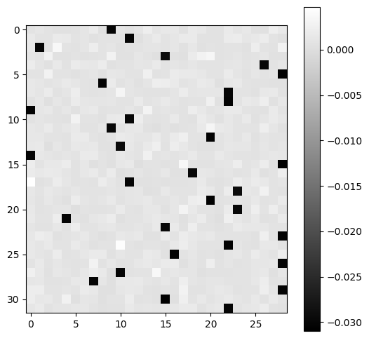
We can now compute the partial derivatives of the loss with respect to the logits of the output layer.
# backward pass

# -----------------
dlogits = F.softmax(logits, dim=1)
dlogits[range(n), Yb] -= 1
dlogits /= n
# -----------------

cmp('logits', dlogits, logits)
logits | exact: False | approximate: True | maxdiff: 5.122274160385132e-09
plt.figure(figsize=(6, 6))
plt.imshow(dlogits.detach(), cmap='gray')
plt.colorbar()
plt.show();
Batch Normalization
Batch normalization is a crucial technique that normalizes the input of a layer to improve training stability and speed up convergence. It works by normalizing activations within each mini-batch.
Mathematical Definition
The batch normalization operation is defined as:
\[\hat{x} = \frac{x - \mu}{\sigma}\]where:
- \(x\) is the input activation
- \(\mu\) is the mean of the input across the batch
- \(\sigma\) is the standard deviation of the input across the batch
- \(\hat{x}\) is the normalized output
Why It Works
- Internal Covariate Shift: Batch norm reduces the internal covariate shift problem, where the distribution of activations changes as parameters update
- Gradient Flow: It helps maintain good gradient flow through the network by keeping activations in a reasonable range
- Regularization: It has a slight regularizing effect due to the noise introduced by batch statistics
Learnable Parameters
In practice, batch normalization includes learnable scale (\(\gamma\)) and shift (\(\beta\)) parameters:
\[y = \gamma \hat{x} + \beta\]This allows the network to learn whether normalization is beneficial and to what degree.
# backprop through batchnorm but all in one go
# BatchNorm paper: https://arxiv.org/abs/1502.03167

# forward pass

# before:
# bnmeani = 1/n*hprebn.sum(0, keepdim=True)
# bndiff = hprebn - bnmeani
# bndiff2 = bndiff**2
# bnvar = 1/(n-1)*(bndiff2).sum(0, keepdim=True) # note: Bessel's correction (dividing by n-1, not n)
# bnvar_inv = (bnvar + 1e-5)**-0.5
# bnraw = bndiff * bnvar_inv
# hpreact = bngain * bnraw + bnbias

# now:
hpreact_fast = bngain * (hprebn - hprebn.mean(0, keepdim=True)) / torch.sqrt(hprebn.var(0, keepdim=True, unbiased=True) + 1e-5) + bnbias
print('max diff:', (hpreact_fast - hpreact).abs().max())
max diff: tensor(3.5763e-07, grad_fn=<MaxBackward1>)
# backward pass

# before we had:
# dbnraw = bngain * dhpreact
# dbndiff = bnvar_inv * dbnraw
# dbnvar_inv = (bndiff * dbnraw).sum(0, keepdim=True)
# dbnvar = (-0.5*(bnvar + 1e-5)**-1.5) * dbnvar_inv
# dbndiff2 = (1.0/(n-1))*torch.ones_like(bndiff2) * dbnvar
# dbndiff += (2*bndiff) * dbndiff2
# dhprebn = dbndiff.clone()
# dbnmeani = (-dbndiff).sum(0)
# dhprebn += 1.0/n * (torch.ones_like(hprebn) * dbnmeani)

# calculate dhprebn given dhpreact (i.e. backprop through the batchnorm)

# -----------------
dhprebn = bngain*bnvar_inv/n * (n*dhpreact - dhpreact.sum(0) - n/(n-1)*bnraw* (dhpreact*bnraw).sum(0))
# -----------------

cmp('hprebn', dhprebn, hprebn) # I can only get approximate to be true, my maxdiff is 9e-10
hprebn | exact: False | approximate: True | maxdiff: 9.313225746154785e-10
Model Training
Now that we have implemented and validated our manual backward pass, let’s use it to train the neural network. This section demonstrates how to integrate our manual gradient computation into a complete training loop.
Training Strategy
We’ll use our manual gradients instead of PyTorch’s automatic differentiation to update the model parameters. This gives us complete control over the training process and validates that our manual implementation is correct.
# Train the MLP neural network using our manual backward pass implementation

# Initialize model parameters for training
# We'll use a larger model than before to see better training dynamics
n_embd = 10      # Character embedding dimension (how rich each character representation is)
n_hidden = 200   # Number of neurons in hidden layer (increased from 64 for better capacity)

# Set random seed for reproducible training
g = torch.Generator().manual_seed(2147483647)

# Initialize embedding matrix: maps each character to a learned vector
C = torch.randn((vocab_size, n_embd), generator=g)

# Initialize first layer (hidden layer) weights and bias
# Use Xavier/Glorot initialization for better gradient flow
W1 = torch.randn((n_embd * CONTEXT_SIZE, n_hidden), generator=g) * (5/3)/((n_embd * CONTEXT_SIZE)**0.5)
b1 = torch.randn(n_hidden, generator=g) * 0.1

# Initialize second layer (output layer) weights and bias
# Use smaller weights for output layer to prevent saturation
W2 = torch.randn((n_hidden, vocab_size), generator=g) * 0.1
b2 = torch.randn(vocab_size, generator=g) * 0.1

# Initialize batch normalization parameters
# Start with scale near 1 and bias near 0 for stable initial behavior
bngain = torch.randn((1, n_hidden)) * 0.1 + 1.0
bnbias = torch.randn((1, n_hidden)) * 0.1

# Collect all parameters for easy access during training
parameters = [C, W1, b1, W2, b2, bngain, bnbias]

# Display total parameter count to understand model complexity
print(f"Total parameters: {sum(p.nelement() for p in parameters):,}")

# Enable gradient tracking for all parameters
for p in parameters:
    p.requires_grad = True

# Training hyperparameters
max_steps = 200000    # Total number of training iterations
batch_size = 32       # Number of samples per batch
n = batch_size        # Convenience variable for batch size
lossi = []            # List to track loss history for plotting

# Training loop using our manual backward pass
# Note: We use torch.no_grad() for efficiency since we're computing gradients manually
# This prevents PyTorch from building computation graphs for the forward pass
with torch.no_grad():

    # Main training loop
    for i in range(max_steps):

        # Step 1: Construct mini-batch
        # Randomly sample batch_size training examples
        ix = torch.randint(0, X_train.shape[0], (batch_size,), generator=g)
        Xb, Yb = X_train[ix], Y_train[ix]  # Input contexts and target characters

        # Step 2: Forward pass through the network
        # This is the same forward pass we implemented earlier

        # Embed characters into learned vector representations
        emb = C[Xb]  # Look up embeddings for each character in the context

        # Concatenate context embeddings into a single vector per sample
        embcat = emb.view(emb.shape[0], -1)  # Flatten context dimension

        # First linear transformation (hidden layer)
        hprebn = embcat @ W1 + b1  # Pre-activation values

        # Batch normalization layer
        # -------------------------------------------------------------
        # Calculate batch statistics
        bnmean = hprebn.mean(0, keepdim=True)                    # Mean across batch
        bnvar = hprebn.var(0, keepdim=True, unbiased=True)       # Variance across batch
        bnvar_inv = (bnvar + 1e-5)**-0.5                        # Inverse std dev
        bnraw = (hprebn - bnmean) * bnvar_inv                    # Normalize
        hpreact = bngain * bnraw + bnbias                        # Scale and shift
        # -------------------------------------------------------------

        # Apply non-linear activation function
        h = torch.tanh(hpreact)  # Hidden layer activations

        # Final linear transformation (output layer)
        logits = h @ W2 + b2  # Unnormalized character probabilities

        # Compute cross-entropy loss
        loss = F.cross_entropy(logits, Yb)  # Loss function

        # Step 3: Manual backward pass (our implementation!)
        # Clear any existing gradients since we're computing them manually
        for p in parameters:
            p.grad = None

        # Note: We don't call loss.backward() since we're computing gradients manually
        # This gives us complete control over the gradient computation process

        # Manual backpropagation through each layer
        # -----------------

        # Start with the gradient of the loss with respect to logits
        # This is the derivative of cross-entropy loss: dL/dlogits = softmax(logits) - targets
        dlogits = F.softmax(logits, 1)                    # Get probabilities
        dlogits[range(n), Yb] -= 1                        # Subtract 1 for target positions
        dlogits /= n                                       # Average over batch

        # Backpropagate through output layer (W2, b2)
        dh = dlogits @ W2.T                               # Gradient w.r.t. hidden activations
        dW2 = h.T @ dlogits                               # Gradient w.r.t. output weights
        db2 = dlogits.sum(0)                              # Gradient w.r.t. output bias

        # Backpropagate through tanh activation
        dhpreact = (1.0 - h**2) * dh                      # Derivative of tanh: 1 - tanh²(x)

        # Backpropagate through batch normalization
        dbngain = (bnraw * dhpreact).sum(0, keepdim=True) # Gradient w.r.t. scale parameter
        dbnbias = dhpreact.sum(0, keepdim=True)           # Gradient w.r.t. shift parameter

        # Use our optimized batch norm backprop formula
        dhprebn = bngain*bnvar_inv/n * (n*dhpreact - dhpreact.sum(0) - n/(n-1)*bnraw*(dhpreact*bnraw).sum(0))

        # Backpropagate through first layer (W1, b1)
        dembcat = dhprebn @ W1.T                          # Gradient w.r.t. concatenated embeddings
        dW1 = embcat.T @ dhprebn                          # Gradient w.r.t. hidden weights
        db1 = dhprebn.sum(0)                              # Gradient w.r.t. hidden bias

        # Backpropagate through embedding layer
        demb = dembcat.view(emb.shape)                    # Reshape gradient to embedding dimensions
        dC = torch.zeros_like(C)                          # Initialize embedding gradient matrix

        # Scatter gradients back to embedding matrix
        # Since multiple positions may use the same character, we accumulate gradients
        for k in range(Xb.shape[0]):      # For each sample in batch
            for j in range(Xb.shape[1]):  # For each position in context
                ix = Xb[k,j]              # Get character index at this position
                dC[ix] += demb[k,j]       # Accumulate gradient for this character

        # Collect all computed gradients in the same order as parameters
        grads = [dC, dW1, db1, dW2, db2, dbngain, dbnbias]
        # -----------------

        # Step 4: Parameter updates using our manual gradients
        # Implement learning rate scheduling: start with higher LR, then reduce
        lr = 0.1 if i < 100000 else 0.01  # Step learning rate decay

        # Update each parameter using its corresponding manual gradient
        # Note: We use our manual gradients instead of PyTorch's automatic gradients
        for p, grad in zip(parameters, grads):
            # Old way (using PyTorch gradients): p.data += -lr * p.grad
            # New way (using our manual gradients): p.data += -lr * grad
            p.data += -lr * grad  # Gradient descent update rule

        # Step 5: Monitor training progress
        # Print loss every 10,000 steps to track convergence
        if i % 10000 == 0:
            print(f'{i:7d}/{max_steps:7d}: {loss.item():.4f}')

        # Store loss history for later analysis and plotting
        # Use log10 scale to better visualize the loss reduction
        lossi.append(loss.log10().item())
        0/ 200000: 3.8111
    10000/ 200000: 1.5936
    20000/ 200000: 2.1010
    30000/ 200000: 1.4711
    40000/ 200000: 2.1248
    50000/ 200000: 1.6181
    60000/ 200000: 1.7196
    70000/ 200000: 1.2026
    80000/ 200000: 1.3953
    90000/ 200000: 1.4356
    100000/ 200000: 1.4518
    110000/ 200000: 1.2661
    120000/ 200000: 1.2207
    130000/ 200000: 1.4259
    140000/ 200000: 1.5294
    150000/ 200000: 1.5008
    160000/ 200000: 1.4570
    170000/ 200000: 1.6469
    180000/ 200000: 1.1593
    190000/ 200000: 1.3232
# Calibrate batch normalization parameters after training
# During training, batch norm uses statistics from each mini-batch
# For inference, we want to use statistics from the entire training set for consistency

with torch.no_grad():  # No need to track gradients during inference
    # Pass the entire training set through the network to compute global statistics
    emb = C[X_train]                    # Embed all training characters
    embcat = emb.view(emb.shape[0], -1) # Concatenate embeddings
    hpreact = embcat @ W1 + b1          # Compute pre-activations

    # Calculate mean and variance across the entire training set
    # These will be used for inference instead of batch-specific statistics
    bnmean = hpreact.mean(0, keepdim=True)                    # Global mean per feature
    bnvar = hpreact.var(0, keepdim=True, unbiased=True)       # Global variance per feature
# Evaluate model performance on training and validation sets
# This function computes the loss on different data splits for model assessment

@torch.no_grad()  # Disable gradient tracking during evaluation for efficiency
def split_loss(split):
    """
    Compute loss on a specific data split (train/val/test).

    Args:
        split (str): Data split to evaluate ('train', 'val', or 'test')

    Returns:
        None: Prints the loss for the specified split
    """
    # Select the appropriate data split
    x, y = {
        'train': (X_train, Y_train),
        'val': (X_dev, Y_dev),
        'test': (X_test, Y_test),
    }[split]

    # Forward pass through the network (same as training but without gradients)
    emb = C[x]                                    # Embed characters: (N, context_size, embedding_dim)
    embcat = emb.view(emb.shape[0], -1)           # Concatenate: (N, context_size * embedding_dim)
    hpreact = embcat @ W1 + b1                    # Linear transformation

    # Apply batch normalization using global statistics (not batch-specific)
    # This ensures consistent behavior during inference
    hpreact = bngain * (hpreact - bnmean) * (bnvar + 1e-5)**-0.5 + bnbias

    h = torch.tanh(hpreact)                       # Non-linear activation: (N, hidden_size)
    logits = h @ W2 + b2                          # Output layer: (N, vocab_size)

    # Compute cross-entropy loss
    loss = F.cross_entropy(logits, y)

    # Display the result
    print(f"{split}: {loss.item():.4f}")

# Evaluate on training and validation sets
# Training loss should be lower than validation loss (indicating some overfitting is normal)
split_loss('train')
split_loss('val')
train 1.3426601886749268
val 1.3950341939926147