Visit the U.S. National Parks

NationalParks
Motivation
The first National Park in the United States that I visited was Congaree National Park in South Carolina in 2018. I was immediately fascinated by the natural landscape and the vast biodiversity that I saw within the park. Since that time, I have visited a total of 5 National Parks across the US and I do not plan on stopping anytime soon. Through this project, I will combine my passion for National Parks and machine learning to create a useful tool that will help those who wish to understand the National Park System better and explore America’s “Best Idea”.
Goal
Yellowstone National Park was established as the first National Park in 1872. Since then, 61 Parks have been added to the US National Park System. The National Parks are the best illustration of what the American ecosystem has to offer. Every year, these locations welcome more than 80 millions visitors. The goal of usaparks.io is to transport visitors into the best locations of each park. By using machine learning and clustering techniques, the application identifies the most photographed locations and gives the user the possibility to access some of these photographs. This application can be used as a tool to help you plan your upcoming trip to a National Park by showing you the most popular attractions or simply to give you virtual access to what these Parks have to offer.
Interface
Data
The National Parks information was retrieved from the Wikipedia page. In order to make this project feasible, we needed access to a large dataset of geolocalized photographs. The website data was scrapped using the popular python library BeautifulSoup. Once the initial information has been gathered for all 62 National Parks, the park boundaries were obtained from the official National Park Service Website. The obtained Geojson files are used to identify pictures that are taken inside each park. The photographs were obtained using the Flickr API. For each park, we create a bounding box using the maximum and minimum longitude and latitude obtained from the Geojson files.
Clustering
In order to identify the most visited locations, we used Density-Based Spatial Clustering of Applications with Noise (DBSCAN). The longitude and latitude of each photograph are used to cluster the photos. The DBSCAN algorithm takes two parameters. The first one in the maximum distance used to search neighbors and the second one is the minimum number of neighbors to be contained within the maximum distance to be considered a cluster.
In order to identify the most visited locations, we used Density-Based Spatial Clustering of Applications with Noise (DBSCAN). The longitude and latitude of each photograph are used to cluster the photos. The DBSCAN algorithm takes two parameters. The first one in the maximum distance used to search neighbors and the second one is the minimum number of neighbors to be contained within the maximum distance to be considered a cluster.
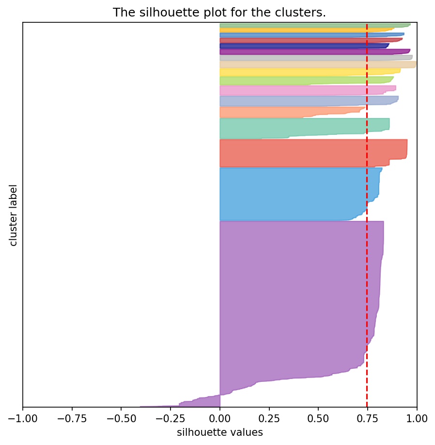
In order to find the best parameters, we define a metric of interest called the silhouette score.
For a data point \(i \in C_{i}\) (data point \(i\) in the cluster \(C_{i}\)), let
\(a(i) = \frac{1}{|C_i| - 1} \sum_{j \in C_i, i \neq j} d(i, j)\)
be the mean distance between \(i\) and all other data points in the same cluster, where \(d(i, j)\) is the distance between data points \(i\) and \(j\) in the cluster \(C_i\) (we divide by \(|C_i| - 1\) because we do not include the distance \(d(i, i)\) in the sum). We can interpret \(a(i)\) as a measure of how well \(i\) is assigned to its cluster (the smaller the value, the better the assignment). We then define the mean dissimilarity of point \(i\) to some cluster \(C_k\) as the mean of the distance from \(i\) to all points in \(C_k\) (where \(C_k \neq C_i\)). For each data point \(i \in C_i\), we now define :
\(b(i) = \min_{k \neq i} \frac{1}{|C_k|} \sum_{j \in C_k} d(i, j)\)
to be the ‘‘smallest’’ (hence the \(\min\) operator in the formula) mean distance of \(i\) to all points in any other cluster, of which \(i\) is not a member. The cluster with this smallest mean dissimilarity is said to be the “neighboring cluster” of \(i\) because it is the next best fit cluster for point \(i\). We now define a ‘‘silhouette’’ (value) of one data point \(i\) :
\(s(i) = \frac{b(i) - a(i)}{\max\{a(i),b(i)\}} , if |C_i| > 1\) and : \(s(i)=0 , if |C_i|=1\)
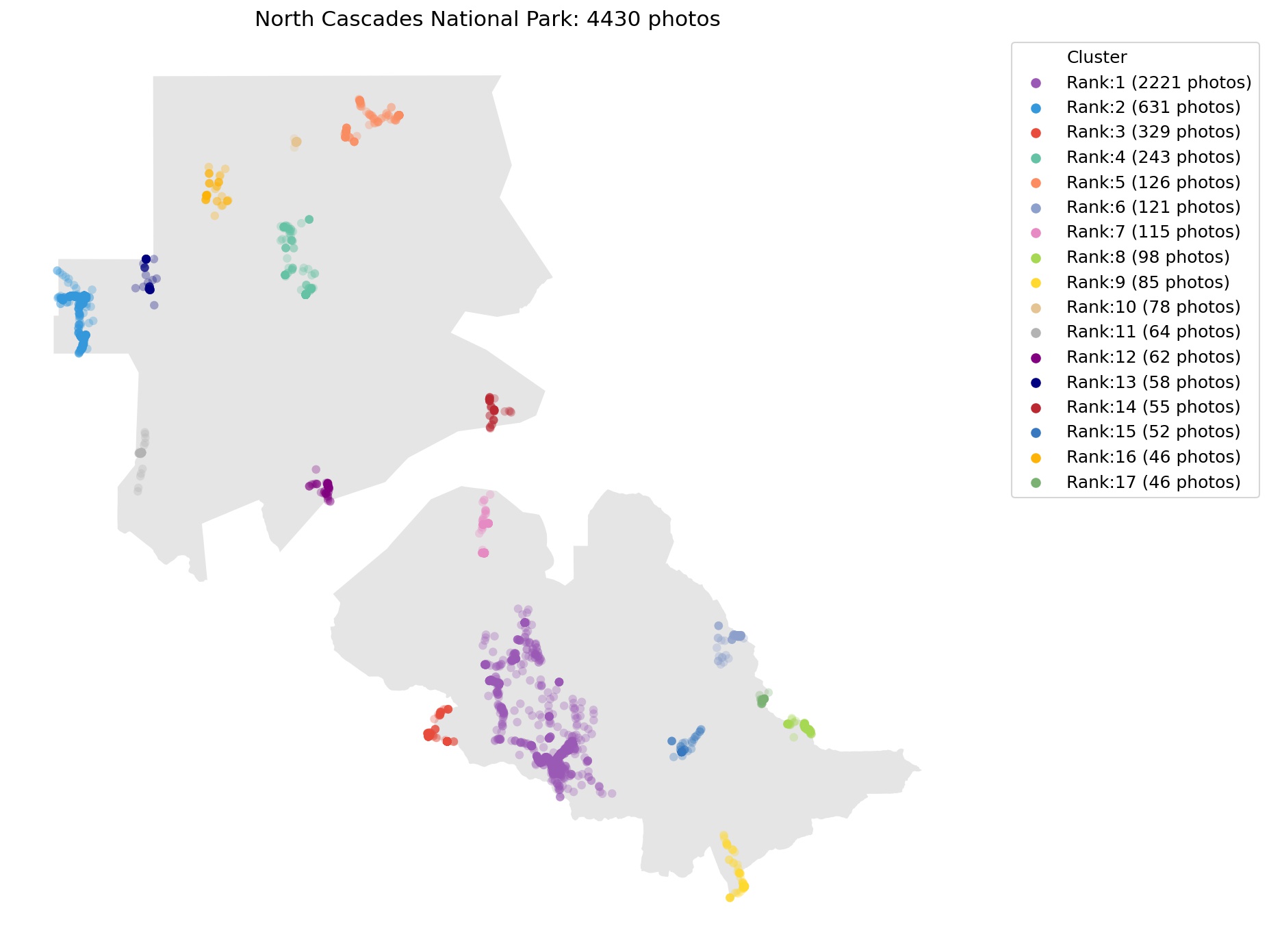
For each park, the parameters of the DBSCAN model are optimized. Below is an example of the clustering results for the North Cascade National Park.
 |  |
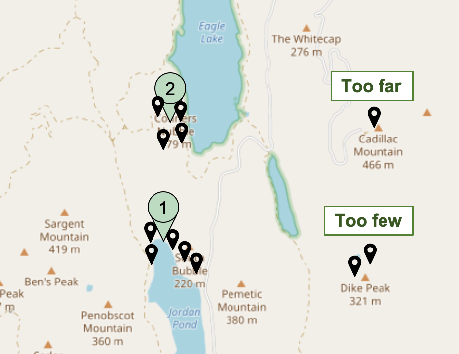
As depicted on the image below, two clusters were obtained from the photo distribution with a minimum samples equal to 3. With four photos, cluster 1 is the most visited location. The two images on the top-right were not clustered because they do not meet the minimum sample requirement. The single photo on the bottom right is not assigned to any cluster as it is too isolated.

Tags
When a photo is uploaded by a user on Flickr, tags can be added manually to the post. Tags consist of words that are relevant to the photo (location, photo content). The tags are compiled for each cluster and sorted using the Term Frequency–Inverse Document Frequency (tf-idf). This summary of the most import tags is then provided on the cluster page to help describe the location corresponding to the cluster. The term frequency is defined as the number of times that term \(t\) occurs in document \(d\):
\(tf(t,d)=f_{t,d} \Bigg/ {\sum_{t' \in d}{f_{t',d}}}\) where:
\(d\) is the document (list of tags associated to an image)
\(t\) is the current tag
The inverse document frequency is the logarithmically scaled inverse fraction of the documents that contain the word (obtained by dividing the total number of documents by the number of documents containing the term, and then taking the logarithm of that quotient):
\(\mathrm{idf}(t, D) = \log \frac{N}{|\{d \in D: t \in d\}|}\)
where
\(N\): total number of documents in the corpus \(N = {|D|}\)
\(|\{d \in D: t \in d\}|\) : number of documents where the term \(t\) appears (i.e., \(\mathrm{tf}(t,d) \neq 0\)). If the term is not in the corpus, this will lead to a division-by-zero. It is therefore common to adjust the denominator to \(1 + |\{d \in D: t \in d\}|\).
Then tf–idf is calculated as:
\(\mathrm{tfidf}(t,d,D) = \mathrm{tf}(t,d) \cdot \mathrm{idf}(t, D)\)
Architecture
