A Take on MNIST
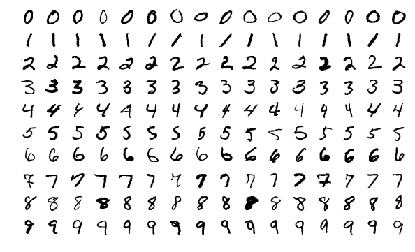
In this Notebook, we will built a progressively more complex model to predict hand-written digits stored in the famous MNIST dataset. The goal is to understand the effects of our modeling choices and how the performances of our models can be optimized. We will start by building the simplest model (mutinomial logistic regression) and incrementally increase the complexity the approach in order to improve the accuracy of our predictions.
0. Load data
1. Exploratory Analysis
1.a. Classes to predict
1.b. Input features
1.c Dataset Size
2. Logistic Regression
2.a Theory
2.b Simple example
2.c Logistic Regression on MNIST (no normalization)
2.d Logistic Regression on MNIST (Lasso and Ridge regularizations)
3. Deep Neural Networks (DNN)
4. Convolutional Networks (CNN)
5. Convolutional Networks (CNN) with data augmentation
6. Conclusion and Kaggle Submittal
# load libraries
import numpy as np
import pandas as pd

# plotting tools
import matplotlib.pyplot as plt
import seaborn as sns
plt.style.use('ggplot')
%matplotlib inline

import tensorflow as tf
print('Tensforflow:',tf.__version__)
from tensorflow import keras
print('Keras:', keras.__version__)
from keras.utils.np_utils import to_categorical
from tensorflow.keras.optimizers import RMSprop
from tensorflow.keras.callbacks import ReduceLROnPlateau

# models
import sklearn
print('scikit-learn',sklearn.__version__)
from sklearn.linear_model import SGDClassifier, LogisticRegression
from sklearn.model_selection import GridSearchCV

# metrics
from sklearn.metrics import accuracy_score, confusion_matrix
from sklearn.utils.multiclass import unique_labels

# tools
import TAD_tools # personal tools and functions
Tensforflow: 1.14.0
Keras: 2.2.4-tf
scikit-learn 0.21.2

Using TensorFlow backend.
# store results
df_results = pd.DataFrame(columns=['Model','Training accuracy','Testing accuracy'])
0. Load data
The MNIST is a famous dataset. It can be retrieved directly from the keras library. The dataset will be divided into two sets. A training set will be used to train our model while the test set will be used to evaluate the performance of the model when subjected to unknown data.
# load data
mnist = tf.keras.datasets.mnist

# create a train and a test set
(X_train, Y_train),(X_test, Y_test) = mnist.load_data()
1. Exploratory Analysis
Before rushing to the modeling aspect of this problem, it is essential to explore the dataset. During this step, we are primarily focused on the followings:
a. What are the classes to predict?
b. What does the input data look like?
c. How big is the dataset?
d. Are there any missing values or outliers?
1.a. Classes to predict
As previously stated, the MNIST dataset consists of a collection of images of single hand-written digits (0 through 9).
# number of classes and unique classes
print("The model consists of {} classes. They are labeled as:\n".format(len(np.unique(Y_train))))
print(np.unique(Y_train))
The model consists of 10 classes. They are labeled as:

[0 1 2 3 4 5 6 7 8 9]
1.b. Input features
print("Each of the input image is {} by {} pixels.".format(X_train[0].shape[0],X_train[0].shape[1]))
print("The grayscale varies from {} to {}.".format(X_train.min(),X_train.max()))
Each of the input image is 28 by 28 pixels.
The grayscale varies from 0 to 255.
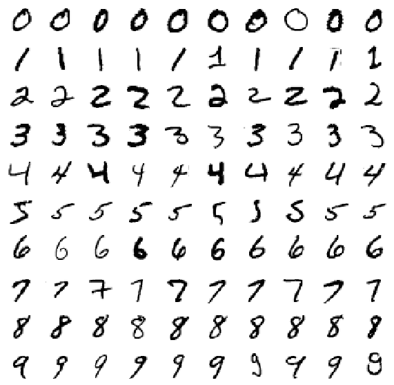
Let’s now plot a few images of each classes to understand what we are dealing with.
# unique classes
unique_classes = np.unique(Y_train)

# create plot figure
fig, axes = plt.subplots(10,10,figsize=(10,10))


# loop over the classes and plots a few randomly selected images
for idx, digit in enumerate(unique_classes):
    selected_images = X_train[Y_train==digit][0:10]

    for k in range(0,10):
        axes[digit,k].imshow(selected_images[k],cmap='Greys', vmin=0, vmax=255)
        axes[digit,k].axis('off')
1.c Dataset Size
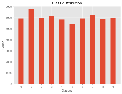
When working on a classification problem, it is essential to know if our training data is well distributed amongst the different classes.
print("There are {} training examples and {} test examples.".format(X_train.shape[0],X_test.shape[0]))
There are 60000 training examples and 10000 test examples.
# plot histogram of digit class distribution
fig, ax = plt.subplots(figsize=(8,6))
ax.hist(Y_train,density=False,rwidth=0.5,align='left',bins=list(range(11)))
ax.set_xticks([x for x in np.unique(Y_train)])
ax.set_xticklabels([x for x in np.unique(Y_train)])
ax.set_title('Class distribution')
ax.set_xlabel('Classes')
ax.set_ylabel('Count');
# list class distributions
print('Class distribution in dataset (%):')
pd.Series(Y_train).value_counts().sort_index() / Y_train.shape[0] * 100.0
Class distribution in dataset (%):

0     9.871667
1    11.236667
2     9.930000
3    10.218333
4     9.736667
5     9.035000
6     9.863333
7    10.441667
8     9.751667
9     9.915000
dtype: float64
The class distribution is even enough to consider the dataset ready for use. It is essential to establish how classes are distributed in order to define our accuracy baseline. For instance, let’s consider a model used to predict if a coin will land on head or tail. If our dataset contains 10% heads and 90% tails then a dummy model predicting “tail” for any input will have an accuracy of 90%.
NORMALIZATION:
In order to improve the performance of our models, we will normalized the pixel values so they fall between 0 and 1.
# normalize pixel value to range between 0 and 1 instead of ranging between 0 and 255
X_train = X_train / 255.0
X_test = X_test / 255.0
2. Logistic Regression
2.a Theory
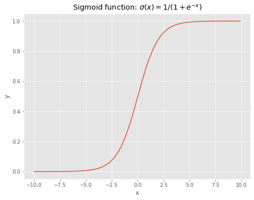
The first model will consist of a simple logistic regression. The logistic regression takes its origins from the linear regression. The linear regression (\(L\)) is coupled with the sigmoid function (\(\sigma\)). They are defined as:
\[L(x) = \beta_{0} + \sum_{n=1}^{N} \beta_{n} * x_{n}\]and
\[\sigma(x) = \frac{1}{1+e^{-x}}\]# create sigmoid function
x = np.arange(-10,10,0.1)
y = 1 / (1+np.exp(-x))
# plot sigmoid
fig, ax = plt.subplots(figsize=(8,6))
ax.plot(x,y)
ax.set_xlabel('x')
ax.set_ylabel('y')
ax.set_title('Sigmoid function: $$\sigma(x)=1/(1+e^{-x})$$');
2.b Simple example
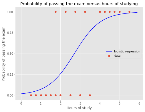
Let’s consider a simple example. In a class of 20 students, we asked how many hours were spent studying on a test. We collect the data along with the results of the test. For each of the 20 students, we have a record containing the number of hours spent studying and whether the student pass the test.
# data
x = np.array([0.50,0.75,1.00,1.25,1.50,1.75,1.75,2.00,2.25,
              2.50,2.75,3.00,3.25,3.50,4.00,4.25,4.50,4.75,5.00,5.50]).reshape(-1,1)
y = np.array([0,0,0,0,0,0,1,0,1,0,1,0,1,0,1,1,1,1,1,1])

# create logistic regression
lr = LogisticRegression(penalty='l2',C=10**6,solver='lbfgs')

# train model on original data
lr.fit(x,y)

# generate new test data
x_test = np.arange(0,6,0.1).reshape(-1,1)
# predict the probability of passing the test
y_test_pred = lr.predict_proba(x_test)[:,1]

# plot data
fig, ax = plt.subplots(figsize=(8,6))
ax.scatter(x,y,label='data')
ax.set_xlabel('Hours of study')
ax.set_ylabel('Probability of passing the exam')
ax.set_title('Probability of passing the exam versus hours of studying')
ax.plot(x_test,y_test_pred,c='blue',label='logistic regression')
ax.set_yticks([0,0.25,0.50,0.75,1.0])
ax.legend(loc=7);
Conclusion:
From the above plot, the logistic regression will predict a student will pass the test if he/she studied for more than ~2.6h with a probability greater than 0.5.
2.c Logistic Regression on MNIST (no regularization)
The main difference between the example previously presented and the MNIST dataset is that the test studying example was a binary classification problem. Since the MNIST dataset contains 10 classes, the algorithm needs to be adjusted. The model used for such cases is called multinomial logistic regression. To put it simply, this problem can be solved by dividing it into K-1 regressions where K is the number of classes. Each regression will compute a score which defines the probability of one example to belong to class k. In order to make the predictions, the results obtained by the K-1 models are combined and the one giving the highest score is used to defined the predicted class.
The \(softmax\) function is used to compute the probability of belonging to each class. It is defined as:
\[\sigma(z_{i}) = \frac{e^{z_{i}}}{\sum_{i=1}^{K}e^{z_{i}}}\]Note: The Logistic Regression model computes the analytical solution by inverting matrices. Due to the large size of our training matrix, the analytical solution requires a lot of computing power to be run quickly. Instead, we will use the Stochastic Gradient Descent (SGD) method to approach the analytical solution. The SGD computes the partial derivatives of the cost function with respect to the model parameters. For each iteration, the parameters are updated based on these partial derivatives.
# create model
sgd_clf = SGDClassifier(loss='log', penalty=None, max_iter=20000, learning_rate='optimal', eta0=0.01, n_jobs=4)

# train the model
sgd_clf.fit(X_train.reshape(X_train.shape[0],-1),Y_train)

# make predictions and compute accuracies
Y_train_pred = sgd_clf.predict(X_train.reshape(X_train.shape[0],-1))
Y_test_pred = sgd_clf.predict(X_test.reshape(X_test.shape[0],-1))

acc_train = accuracy_score(Y_train,Y_train_pred)
acc_test = accuracy_score(Y_test,Y_test_pred)

print('The accuracy on the training set is: \t{:.3f}%'.format(acc_train * 100))
print('The accuracy on the test set is: \t{:.3f}%'.format(acc_test * 100))
The accuracy on the training set is: 	91.145%
The accuracy on the test set is: 	89.870%
# store results
df_results = df_results.append({'Model':"Log Reg",'Training accuracy':acc_train,'Testing accuracy':acc_test},ignore_index=True)
2.d Logistic Regression on MNIST (Lasso and Ridge regularizations)
In order to avoid overfitting, we will now incorporate some regularization in our model. There are two types of regularizations:
- \(l1\) type (Lasso)
- \(l2\) type (Ridge)
The idea behind these two methods is the same, avoid large coefficients in the regression and distribute the predictive power of the model over a larger subset of coefficients. The Lasso normalization for a simple linear regression can be defined as the following problem to minimize:
\[\min_{ \beta_0, \beta } \left\{ \frac{1}{N} \sum_{i=1}^N (y_i)*log(\beta_0 - x_i^T \beta) \right\} \text{ subject to } \sum_{j=1}^p |\beta_j| \leq t.\]It because of the nature of the absolute value, the Lasso regularization tends to drop the coefficients of the model to 0.
The Ridge normalization for a simple linear regression can be defined as the following problem to minimize:
\[\min_{ \beta_0, \beta } \left\{ \frac{1}{N} \sum_{i=1}^N (y_i)*log(\beta_0 - x_i^T \beta) \right\} \text{ subject to } \sum_{j=1}^p \beta_j^{2} \leq t.\]Note that both of these methods are defined using a parameter \(t\) where \(t\) is the regularization parameter. Smaller values of \(t\) will leads to more regularization.
# Lasso

# create model
lasso = SGDClassifier(loss='log', penalty='l1', max_iter=20000, learning_rate='optimal', eta0=0.01, n_jobs=4, alpha=0.0001)

# train the model
lasso.fit(X_train.reshape(X_train.shape[0],-1),Y_train)

# make predictions and compute accuracies
Y_train_pred = lasso.predict(X_train.reshape(X_train.shape[0],-1))
Y_test_pred = lasso.predict(X_test.reshape(X_test.shape[0],-1))

acc_train = accuracy_score(Y_train,Y_train_pred)
acc_test = accuracy_score(Y_test,Y_test_pred)

print('The accuracy on the training set is: \t{:.3f}%'.format(acc_train*100))
print('The accuracy on the test set is: \t{:.3f}%'.format(acc_test*100))
The accuracy on the training set is: 	91.390%
The accuracy on the test set is: 	90.700%
# store results
df_results = df_results.append({'Model':"Lasso",'Training accuracy':acc_train,'Testing accuracy':acc_test},ignore_index=True)
# Ridge

# create model
ridge = SGDClassifier(loss='log', penalty='l2', max_iter=20000, learning_rate='optimal', eta0=0.01, n_jobs=4, alpha=0.0001)

# train the model
ridge.fit(X_train.reshape(X_train.shape[0],-1),Y_train)

# make predictions and compute accuracies
Y_train_pred = ridge.predict(X_train.reshape(X_train.shape[0],-1))
Y_test_pred = ridge.predict(X_test.reshape(X_test.shape[0],-1))

acc_train = accuracy_score(Y_train,Y_train_pred)
acc_test = accuracy_score(Y_test,Y_test_pred)

print('The accuracy on the training set is: \t{:.3f}%'.format(acc_train*100))
print('The accuracy on the test set is: \t{:.3f}%'.format(acc_test*100))
The accuracy on the training set is: 	92.040%
The accuracy on the test set is: 	91.520%
# store results
df_results = df_results.append({'Model':"Ridge",'Training accuracy':acc_train,'Testing accuracy':acc_test},ignore_index=True)
df_results
| Model | Training accuracy | Testing accuracy | |
|---|---|---|---|
| 0 | Log Reg | 0.91145 | 0.8987 |
| 1 | Lasso | 0.91390 | 0.9070 |
| 2 | Ridge | 0.92040 | 0.9152 |
3. Deep Neural Networks (DNN)
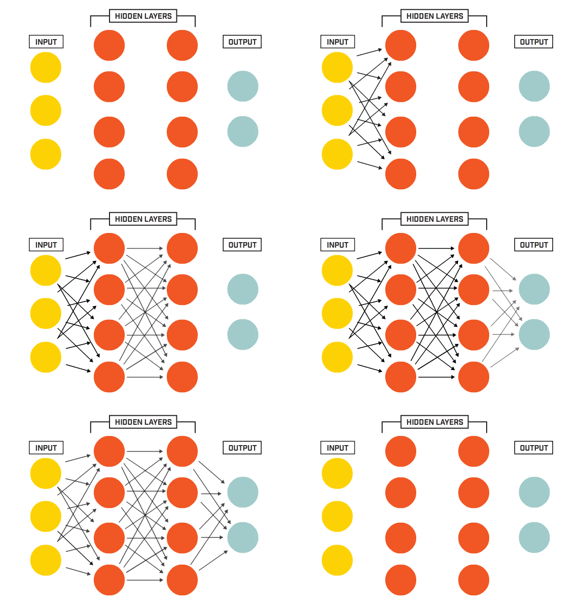
Neural Networks combine the simplicity of simple regression and the power of model combination. A neural network is an ensemble of neurons. Each neuron can be seen as a linear functions. The network is made of neurons arranged in layers. The last layer of the neural network is used to predict the output classes. We begin by creating a neural network of three fully connected layers.
Source: www.kookycoder.com
The architecture of a neural networks is made of three different types of layers. The input layer consists of the properly formatted input data. In our case, we flatten the 28x28 images into a 784-component vector. The output layer consists of a set of neurons (1 neuron for each output class). Finally, the body of the network consists of hidden layers. Each neuron of each layer is connected to each neuron of the next layer.
Source: https://cloud.google.com
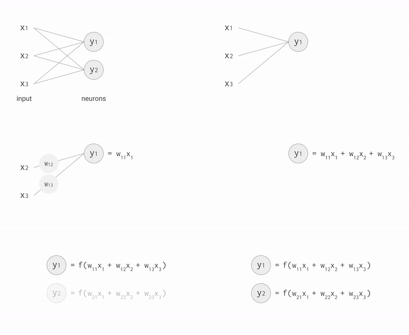
Each neuro is definedd with a set of weights (\(w_ij\)) and an activation function. The role of the activation function is to increase the complexity of the model to capture non-linear behaviors. The most common activation function of the hidden layers is called “Rectified Linear Unit” (RELU) and is defined as \(f(x)=max(x,0)\).
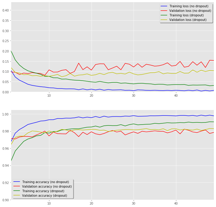
Note: as part of the regularization effort, dropouts are included in the model. The idea behind the use of dropout is to prevent the model from relying too heavily on the same neurons. To do so, a random subset of neurons is deactivated (coefficients set to 0) at each iteration.
# load data
mnist = tf.keras.datasets.mnist

# create a train and a test set
(X_train, Y_train),(X_test, Y_test) = mnist.load_data()
X_train = X_train / 255.0
X_test = X_test / 255.0
# create nn (128->64->32->10)
model_dnn_no_drop = tf.keras.Sequential([
        tf.keras.layers.Flatten(),
        tf.keras.layers.Dense(128,activation='relu'),
        tf.keras.layers.Dense(64,activation='relu'),
        tf.keras.layers.Dense(32,activation='relu'),
        tf.keras.layers.Dense(10,activation='softmax')
        ])

model_dnn_drop = tf.keras.Sequential([
        tf.keras.layers.Flatten(),
        tf.keras.layers.Dense(128,activation='relu'),
        tf.keras.layers.Dropout(0.20),
        tf.keras.layers.Dense(64,activation='relu'),
        tf.keras.layers.Dropout(0.20),
        tf.keras.layers.Dense(32,activation='relu'),
        tf.keras.layers.Dropout(0.20),
        tf.keras.layers.Dense(10,activation='softmax')
        ])
# compile model
model_dnn_no_drop.compile(
        optimizer=tf.keras.optimizers.Adam(),
        loss='sparse_categorical_crossentropy',
        metrics=['acc'],
        lr=0.001
        )

model_dnn_drop.compile(
        optimizer=tf.keras.optimizers.Adam(),
        loss='sparse_categorical_crossentropy',
        metrics=['acc'],
        lr=0.001
        )
# train model
history_dnn_no_drop = model_dnn_no_drop.fit(
        X_train,
        Y_train,
        epochs=50,
        validation_data=(X_test, Y_test)
        )
Train on 60000 samples, validate on 10000 samples
Epoch 1/50
60000/60000 [==============================] - 3s 43us/sample - loss: 0.2561 - acc: 0.9246 - val_loss: 0.1324 - val_acc: 0.9583
Epoch 2/50
60000/60000 [==============================] - 2s 41us/sample - loss: 0.1047 - acc: 0.9678 - val_loss: 0.0972 - val_acc: 0.9714
Epoch 3/50
60000/60000 [==============================] - 2s 41us/sample - loss: 0.0724 - acc: 0.9777 - val_loss: 0.0959 - val_acc: 0.9709
Epoch 4/50
60000/60000 [==============================] - 3s 42us/sample - loss: 0.0570 - acc: 0.9820 - val_loss: 0.0846 - val_acc: 0.9732
Epoch 5/50
60000/60000 [==============================] - 2s 41us/sample - loss: 0.0473 - acc: 0.9848 - val_loss: 0.0918 - val_acc: 0.9739
Epoch 6/50
60000/60000 [==============================] - 2s 42us/sample - loss: 0.0370 - acc: 0.9878 - val_loss: 0.0894 - val_acc: 0.9738
Epoch 7/50
60000/60000 [==============================] - 3s 42us/sample - loss: 0.0316 - acc: 0.9891 - val_loss: 0.0942 - val_acc: 0.9733
Epoch 8/50
60000/60000 [==============================] - 3s 42us/sample - loss: 0.0282 - acc: 0.9904 - val_loss: 0.0915 - val_acc: 0.9756
Epoch 9/50
60000/60000 [==============================] - 2s 41us/sample - loss: 0.0252 - acc: 0.9918 - val_loss: 0.0899 - val_acc: 0.9776
Epoch 10/50
60000/60000 [==============================] - 3s 42us/sample - loss: 0.0234 - acc: 0.9922 - val_loss: 0.0812 - val_acc: 0.9801
Epoch 11/50
60000/60000 [==============================] - 3s 42us/sample - loss: 0.0201 - acc: 0.9933 - val_loss: 0.1076 - val_acc: 0.9744
Epoch 12/50
60000/60000 [==============================] - 3s 42us/sample - loss: 0.0192 - acc: 0.9934 - val_loss: 0.0968 - val_acc: 0.9789
Epoch 13/50
60000/60000 [==============================] - 3s 42us/sample - loss: 0.0162 - acc: 0.9948 - val_loss: 0.0971 - val_acc: 0.9771
Epoch 14/50
60000/60000 [==============================] - 3s 44us/sample - loss: 0.0160 - acc: 0.9947 - val_loss: 0.1052 - val_acc: 0.9769
Epoch 15/50
60000/60000 [==============================] - 3s 44us/sample - loss: 0.0144 - acc: 0.9952 - val_loss: 0.1085 - val_acc: 0.9768
Epoch 16/50
60000/60000 [==============================] - 2s 39us/sample - loss: 0.0148 - acc: 0.9952 - val_loss: 0.0906 - val_acc: 0.9811
Epoch 17/50
60000/60000 [==============================] - 2s 41us/sample - loss: 0.0142 - acc: 0.9956 - val_loss: 0.0995 - val_acc: 0.9782
Epoch 18/50
60000/60000 [==============================] - 3s 44us/sample - loss: 0.0103 - acc: 0.9966 - val_loss: 0.1406 - val_acc: 0.9736
Epoch 19/50
60000/60000 [==============================] - 3s 42us/sample - loss: 0.0145 - acc: 0.9955 - val_loss: 0.1084 - val_acc: 0.9788
Epoch 20/50
60000/60000 [==============================] - 3s 43us/sample - loss: 0.0098 - acc: 0.9964 - val_loss: 0.1224 - val_acc: 0.9760
Epoch 21/50
60000/60000 [==============================] - 3s 44us/sample - loss: 0.0131 - acc: 0.9958 - val_loss: 0.1064 - val_acc: 0.9793
Epoch 22/50
60000/60000 [==============================] - 3s 44us/sample - loss: 0.0094 - acc: 0.9972 - val_loss: 0.1337 - val_acc: 0.9769
Epoch 23/50
60000/60000 [==============================] - 2s 41us/sample - loss: 0.0129 - acc: 0.9959 - val_loss: 0.1373 - val_acc: 0.9759
Epoch 24/50
60000/60000 [==============================] - 3s 43us/sample - loss: 0.0079 - acc: 0.9975 - val_loss: 0.1371 - val_acc: 0.9773
Epoch 25/50
60000/60000 [==============================] - 3s 46us/sample - loss: 0.0114 - acc: 0.9964 - val_loss: 0.1081 - val_acc: 0.9793
Epoch 26/50
60000/60000 [==============================] - 3s 45us/sample - loss: 0.0090 - acc: 0.9970 - val_loss: 0.1165 - val_acc: 0.9808
Epoch 27/50
60000/60000 [==============================] - 3s 47us/sample - loss: 0.0095 - acc: 0.9971 - val_loss: 0.1255 - val_acc: 0.9790
Epoch 28/50
60000/60000 [==============================] - 2s 41us/sample - loss: 0.0100 - acc: 0.9970 - val_loss: 0.1080 - val_acc: 0.9800
Epoch 29/50
60000/60000 [==============================] - 3s 43us/sample - loss: 0.0075 - acc: 0.9976 - val_loss: 0.1395 - val_acc: 0.9756
Epoch 30/50
60000/60000 [==============================] - 3s 43us/sample - loss: 0.0079 - acc: 0.9974 - val_loss: 0.1352 - val_acc: 0.9775
Epoch 31/50
60000/60000 [==============================] - 3s 43us/sample - loss: 0.0057 - acc: 0.9981 - val_loss: 0.1216 - val_acc: 0.9792
Epoch 32/50
60000/60000 [==============================] - 3s 44us/sample - loss: 0.0098 - acc: 0.9974 - val_loss: 0.1379 - val_acc: 0.9774
Epoch 33/50
60000/60000 [==============================] - 3s 45us/sample - loss: 0.0089 - acc: 0.9974 - val_loss: 0.1203 - val_acc: 0.9799
Epoch 34/50
60000/60000 [==============================] - 3s 42us/sample - loss: 0.0073 - acc: 0.9976 - val_loss: 0.1350 - val_acc: 0.9792
Epoch 35/50
60000/60000 [==============================] - 3s 42us/sample - loss: 0.0068 - acc: 0.9980 - val_loss: 0.1311 - val_acc: 0.9797
Epoch 36/50
60000/60000 [==============================] - 3s 44us/sample - loss: 0.0079 - acc: 0.9979 - val_loss: 0.1257 - val_acc: 0.9803
Epoch 37/50
60000/60000 [==============================] - 3s 46us/sample - loss: 0.0066 - acc: 0.9981 - val_loss: 0.1276 - val_acc: 0.9798
Epoch 38/50
60000/60000 [==============================] - 3s 44us/sample - loss: 0.0063 - acc: 0.9983 - val_loss: 0.1328 - val_acc: 0.9798
Epoch 39/50
60000/60000 [==============================] - 3s 44us/sample - loss: 0.0073 - acc: 0.9982 - val_loss: 0.1420 - val_acc: 0.9780
Epoch 40/50
60000/60000 [==============================] - 3s 44us/sample - loss: 0.0062 - acc: 0.9981 - val_loss: 0.1264 - val_acc: 0.9793
Epoch 41/50
60000/60000 [==============================] - 2s 42us/sample - loss: 0.0077 - acc: 0.9978 - val_loss: 0.1293 - val_acc: 0.9812
Epoch 42/50
60000/60000 [==============================] - 3s 42us/sample - loss: 0.0067 - acc: 0.9984 - val_loss: 0.1491 - val_acc: 0.9768
Epoch 43/50
60000/60000 [==============================] - 3s 42us/sample - loss: 0.0052 - acc: 0.9984 - val_loss: 0.1205 - val_acc: 0.9824
Epoch 44/50
60000/60000 [==============================] - 3s 44us/sample - loss: 0.0080 - acc: 0.9980 - val_loss: 0.1248 - val_acc: 0.9810
Epoch 45/50
60000/60000 [==============================] - 2s 40us/sample - loss: 0.0055 - acc: 0.9984 - val_loss: 0.1478 - val_acc: 0.9791
Epoch 46/50
60000/60000 [==============================] - 3s 45us/sample - loss: 0.0090 - acc: 0.9977 - val_loss: 0.1304 - val_acc: 0.9784
Epoch 47/50
60000/60000 [==============================] - 3s 42us/sample - loss: 0.0037 - acc: 0.9987 - val_loss: 0.1472 - val_acc: 0.9800
Epoch 48/50
60000/60000 [==============================] - 3s 43us/sample - loss: 0.0071 - acc: 0.9979 - val_loss: 0.1191 - val_acc: 0.9814
Epoch 49/50
60000/60000 [==============================] - 2s 39us/sample - loss: 0.0044 - acc: 0.9987 - val_loss: 0.1547 - val_acc: 0.9773
Epoch 50/50
60000/60000 [==============================] - 3s 42us/sample - loss: 0.0071 - acc: 0.9979 - val_loss: 0.1536 - val_acc: 0.9786
history_dnn_drop = model_dnn_drop.fit(
        X_train,
        Y_train,
        epochs=50,
        validation_data=(X_test, Y_test)
        )
Train on 60000 samples, validate on 10000 samples
Epoch 1/50
60000/60000 [==============================] - 4s 58us/sample - loss: 0.4191 - acc: 0.8747 - val_loss: 0.1423 - val_acc: 0.9564
Epoch 2/50
60000/60000 [==============================] - 3s 55us/sample - loss: 0.2001 - acc: 0.9453 - val_loss: 0.1186 - val_acc: 0.9643
Epoch 3/50
60000/60000 [==============================] - 3s 58us/sample - loss: 0.1560 - acc: 0.9569 - val_loss: 0.0952 - val_acc: 0.9728
Epoch 4/50
60000/60000 [==============================] - 3s 55us/sample - loss: 0.1311 - acc: 0.9626 - val_loss: 0.0917 - val_acc: 0.9742
Epoch 5/50
60000/60000 [==============================] - 3s 53us/sample - loss: 0.1143 - acc: 0.9681 - val_loss: 0.0838 - val_acc: 0.9742
Epoch 6/50
60000/60000 [==============================] - 3s 56us/sample - loss: 0.1029 - acc: 0.9708 - val_loss: 0.0851 - val_acc: 0.9780
Epoch 7/50
60000/60000 [==============================] - 3s 55us/sample - loss: 0.0967 - acc: 0.9724 - val_loss: 0.0788 - val_acc: 0.9802
Epoch 8/50
60000/60000 [==============================] - 3s 57us/sample - loss: 0.0914 - acc: 0.9745 - val_loss: 0.0798 - val_acc: 0.9798
Epoch 9/50
60000/60000 [==============================] - 3s 50us/sample - loss: 0.0854 - acc: 0.9750 - val_loss: 0.0759 - val_acc: 0.9790
Epoch 10/50
60000/60000 [==============================] - 3s 51us/sample - loss: 0.0756 - acc: 0.9783 - val_loss: 0.0793 - val_acc: 0.9781
Epoch 11/50
60000/60000 [==============================] - 3s 54us/sample - loss: 0.0759 - acc: 0.9777 - val_loss: 0.0763 - val_acc: 0.9801
Epoch 12/50
60000/60000 [==============================] - 3s 53us/sample - loss: 0.0689 - acc: 0.9796 - val_loss: 0.0795 - val_acc: 0.9787
Epoch 13/50
60000/60000 [==============================] - 3s 54us/sample - loss: 0.0687 - acc: 0.9796 - val_loss: 0.0854 - val_acc: 0.9801
Epoch 14/50
60000/60000 [==============================] - 3s 52us/sample - loss: 0.0623 - acc: 0.9814 - val_loss: 0.0737 - val_acc: 0.9821
Epoch 15/50
60000/60000 [==============================] - 3s 51us/sample - loss: 0.0629 - acc: 0.9818 - val_loss: 0.0789 - val_acc: 0.9814
Epoch 16/50
60000/60000 [==============================] - 3s 53us/sample - loss: 0.0595 - acc: 0.9825 - val_loss: 0.0899 - val_acc: 0.9799
Epoch 17/50
60000/60000 [==============================] - 3s 54us/sample - loss: 0.0572 - acc: 0.9829 - val_loss: 0.0767 - val_acc: 0.9815
Epoch 18/50
60000/60000 [==============================] - 3s 50us/sample - loss: 0.0563 - acc: 0.9828 - val_loss: 0.0820 - val_acc: 0.9818
Epoch 19/50
60000/60000 [==============================] - 3s 51us/sample - loss: 0.0544 - acc: 0.9837 - val_loss: 0.0834 - val_acc: 0.9813
Epoch 20/50
60000/60000 [==============================] - 3s 52us/sample - loss: 0.0517 - acc: 0.9846 - val_loss: 0.0878 - val_acc: 0.9817
Epoch 21/50
60000/60000 [==============================] - 3s 51us/sample - loss: 0.0488 - acc: 0.9848 - val_loss: 0.0806 - val_acc: 0.9821
Epoch 22/50
60000/60000 [==============================] - 3s 52us/sample - loss: 0.0471 - acc: 0.9860 - val_loss: 0.0836 - val_acc: 0.9820
Epoch 23/50
60000/60000 [==============================] - 3s 51us/sample - loss: 0.0511 - acc: 0.9847 - val_loss: 0.0907 - val_acc: 0.9810
Epoch 24/50
60000/60000 [==============================] - 3s 52us/sample - loss: 0.0472 - acc: 0.9863 - val_loss: 0.0844 - val_acc: 0.9812
Epoch 25/50
60000/60000 [==============================] - 3s 52us/sample - loss: 0.0438 - acc: 0.9867 - val_loss: 0.0926 - val_acc: 0.9797
Epoch 26/50
60000/60000 [==============================] - 3s 52us/sample - loss: 0.0462 - acc: 0.9865 - val_loss: 0.0956 - val_acc: 0.9801
Epoch 27/50
60000/60000 [==============================] - 3s 55us/sample - loss: 0.0464 - acc: 0.9865 - val_loss: 0.0882 - val_acc: 0.9811
Epoch 28/50
60000/60000 [==============================] - 3s 52us/sample - loss: 0.0419 - acc: 0.9876 - val_loss: 0.0905 - val_acc: 0.9814
Epoch 29/50
60000/60000 [==============================] - 3s 52us/sample - loss: 0.0434 - acc: 0.9861 - val_loss: 0.0871 - val_acc: 0.9819
Epoch 30/50
60000/60000 [==============================] - 3s 50us/sample - loss: 0.0407 - acc: 0.9876 - val_loss: 0.0967 - val_acc: 0.9819
Epoch 31/50
60000/60000 [==============================] - 3s 50us/sample - loss: 0.0391 - acc: 0.9885 - val_loss: 0.0879 - val_acc: 0.9815
Epoch 32/50
60000/60000 [==============================] - 3s 50us/sample - loss: 0.0412 - acc: 0.9874 - val_loss: 0.0829 - val_acc: 0.9816
Epoch 33/50
60000/60000 [==============================] - 3s 50us/sample - loss: 0.0419 - acc: 0.9877 - val_loss: 0.0850 - val_acc: 0.9823
Epoch 34/50
60000/60000 [==============================] - 3s 50us/sample - loss: 0.0399 - acc: 0.9880 - val_loss: 0.0894 - val_acc: 0.9830
Epoch 35/50
60000/60000 [==============================] - 3s 52us/sample - loss: 0.0391 - acc: 0.9882 - val_loss: 0.0937 - val_acc: 0.9818
Epoch 36/50
60000/60000 [==============================] - 3s 53us/sample - loss: 0.0359 - acc: 0.9891 - val_loss: 0.0942 - val_acc: 0.9820
Epoch 37/50
60000/60000 [==============================] - 3s 54us/sample - loss: 0.0373 - acc: 0.9888 - val_loss: 0.0989 - val_acc: 0.9815
Epoch 38/50
60000/60000 [==============================] - 3s 56us/sample - loss: 0.0368 - acc: 0.9893 - val_loss: 0.0880 - val_acc: 0.9829
Epoch 39/50
60000/60000 [==============================] - 3s 53us/sample - loss: 0.0335 - acc: 0.9899 - val_loss: 0.0923 - val_acc: 0.9806
Epoch 40/50
60000/60000 [==============================] - 3s 53us/sample - loss: 0.0349 - acc: 0.9896 - val_loss: 0.0900 - val_acc: 0.9827
Epoch 41/50
60000/60000 [==============================] - 3s 56us/sample - loss: 0.0356 - acc: 0.9897 - val_loss: 0.0900 - val_acc: 0.9828
Epoch 42/50
60000/60000 [==============================] - 3s 53us/sample - loss: 0.0353 - acc: 0.9900 - val_loss: 0.0995 - val_acc: 0.9814
Epoch 43/50
60000/60000 [==============================] - 4s 64us/sample - loss: 0.0360 - acc: 0.9899 - val_loss: 0.0911 - val_acc: 0.9822
Epoch 44/50
60000/60000 [==============================] - 4s 65us/sample - loss: 0.0316 - acc: 0.9906 - val_loss: 0.0916 - val_acc: 0.9817
Epoch 45/50
60000/60000 [==============================] - 3s 51us/sample - loss: 0.0333 - acc: 0.9900 - val_loss: 0.1072 - val_acc: 0.9812
Epoch 46/50
60000/60000 [==============================] - 4s 59us/sample - loss: 0.0330 - acc: 0.9903 - val_loss: 0.0960 - val_acc: 0.9824
Epoch 47/50
60000/60000 [==============================] - 3s 54us/sample - loss: 0.0334 - acc: 0.9900 - val_loss: 0.1060 - val_acc: 0.9808
Epoch 48/50
60000/60000 [==============================] - 3s 55us/sample - loss: 0.0337 - acc: 0.9901 - val_loss: 0.0992 - val_acc: 0.9818
Epoch 49/50
60000/60000 [==============================] - 3s 54us/sample - loss: 0.0298 - acc: 0.9910 - val_loss: 0.1046 - val_acc: 0.9831
Epoch 50/50
60000/60000 [==============================] - 3s 56us/sample - loss: 0.0311 - acc: 0.9909 - val_loss: 0.1033 - val_acc: 0.9829
# evaluate performance
print("Training without dropout = ")
model_dnn_no_drop.evaluate(X_train, Y_train)

print("\nTest without dropout = ")
model_dnn_no_drop.evaluate(X_test, Y_test)
Training without dropout =
60000/60000 [==============================] - 1s 21us/sample - loss: 0.0091 - acc: 0.9975

Test without dropout =
10000/10000 [==============================] - 0s 22us/sample - loss: 0.1536 - acc: 0.9786


[0.15362604289185866, 0.9786]
# evaluate performance
print("Training with dropout = ")
model_dnn_drop.evaluate(X_train, Y_train)

print("\nTest with dropout = ")
model_dnn_drop.evaluate(X_test, Y_test)
Training with dropout =
60000/60000 [==============================] - 1s 22us/sample - loss: 0.0055 - acc: 0.9984

Test with dropout =
10000/10000 [==============================] - 0s 21us/sample - loss: 0.1033 - acc: 0.9829

[0.10325850226903108, 0.9829]
# summary
model_dnn_drop.summary()
Model: "sequential_1"
_________________________________________________________________
Layer (type)                 Output Shape              Param #
=================================================================
flatten_1 (Flatten)          multiple                  0
_________________________________________________________________
dense_4 (Dense)              multiple                  100480
_________________________________________________________________
dropout (Dropout)            multiple                  0
_________________________________________________________________
dense_5 (Dense)              multiple                  8256
_________________________________________________________________
dropout_1 (Dropout)          multiple                  0
_________________________________________________________________
dense_6 (Dense)              multiple                  2080
_________________________________________________________________
dropout_2 (Dropout)          multiple                  0
_________________________________________________________________
dense_7 (Dense)              multiple                  330
=================================================================
Total params: 111,146
Trainable params: 111,146
Non-trainable params: 0
_________________________________________________________________
# Plot the loss and accuracy curves for training and validation
x_values = list(range(len(history_dnn_drop.epoch)))

fig, ax = plt.subplots(2,1,figsize=(12,12))
ax[0].plot(x_values,history_dnn_no_drop.history['loss'], color='b', label="Training loss (no dropout)")
ax[0].plot(x_values,history_dnn_no_drop.history['val_loss'], color='r', label="Validation loss (no dropout)",axes =ax[0])
ax[0].plot(x_values,history_dnn_drop.history['loss'], color='g', label="Training loss (dropout)")
ax[0].plot(x_values,history_dnn_drop.history['val_loss'], color='y', label="Validation loss (dropout)",axes =ax[0])
legend = ax[0].legend(loc='best', shadow=True)
ax[0].set_xlim(1,max(x_values))
ax[0].set_ylim(0,)

ax[1].plot(x_values,history_dnn_no_drop.history['acc'], color='b', label="Training accuracy (no dropout)")
ax[1].plot(x_values,history_dnn_no_drop.history['val_acc'], color='r',label="Validation accuracy (no dropout)")
ax[1].plot(x_values,history_dnn_drop.history['acc'], color='g', label="Training accuracy (dropout)")
ax[1].plot(x_values,history_dnn_drop.history['val_acc'], color='y',label="Validation accuracy (dropout)")
legend = ax[1].legend(loc='best', shadow=True)
ax[1].set_xlim(1,max(x_values))
ax[1].set_ylim(0.9,);
# Plot non-normalized confusion matrix
Y_test_pred = model_dnn_drop.predict(X_test)
Y_test_pred = Y_test_pred.argmax(axis=1)

TAD_tools.plot_confusion_matrix(Y_test, Y_test_pred, classes=np.array([str(x) for x in range(11)]),
                     title='Confusion matrix, without normalization');

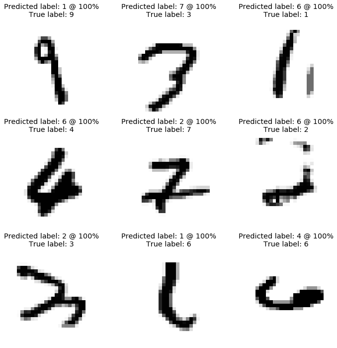
TAD_tools.plot_worst_predictions(model_dnn_drop,X_test,Y_test)
df_results = df_results.append({'Model':"DNN No dropout",
                                'Training accuracy':history_dnn_no_drop.history['acc'][-1],
                                'Testing accuracy':history_dnn_no_drop.history['val_acc'][-1]},ignore_index=True)
df_results = df_results.append({'Model':"DNN Dropout",
                                'Training accuracy':history_dnn_drop.history['acc'][-1],
                                'Testing accuracy':history_dnn_drop.history['val_acc'][-1]},ignore_index=True)
From the plot shown above, we can conclude that our model behaves as expected. Indeed, the prediction errors are made for ambiguous digits.
4. Convolutional Networks (CNN)
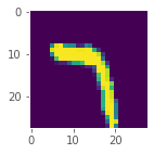
Convolutional Neural Networks were developed with the idea to mimic the human vision. In order to identify objects, our brain first focuses on the overall shape (edges, curves) then the details of the objects are considered. CNN are made of layers, each processes the image to detect pattern. The first layer of the network will detect simple patterns like vertical, horizontal lines, or diagonals. As the transformed images progresses through the network, more complex patterns are identified. The main difference between CNN and DNN is that DNN treats each pixel individually while CNN captures patterns.
The two main types of hidden layers in a CNN are called Convolution and Pooling.
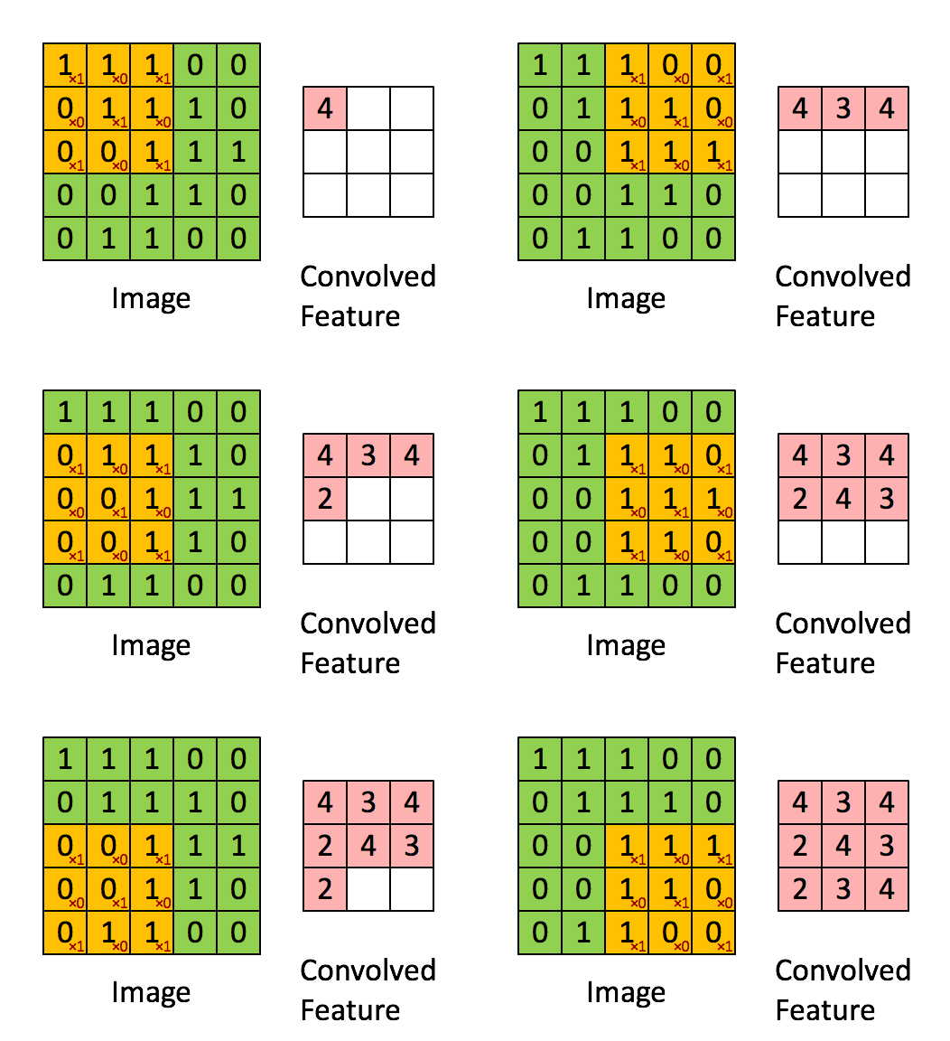
Convolution layers detects pattern while pooling shrink the information. The animation below shows the convolution. A filter (in this case 3x3) travels over the original image. An element wise operation is performed as each elements of the filter is multiplied by the corresponding pixel value and these values are summed together. Without any additional modification, the original 5x5 image is shrunk into a 3x3 image.
Source: https://cdn-images-1.medium.com
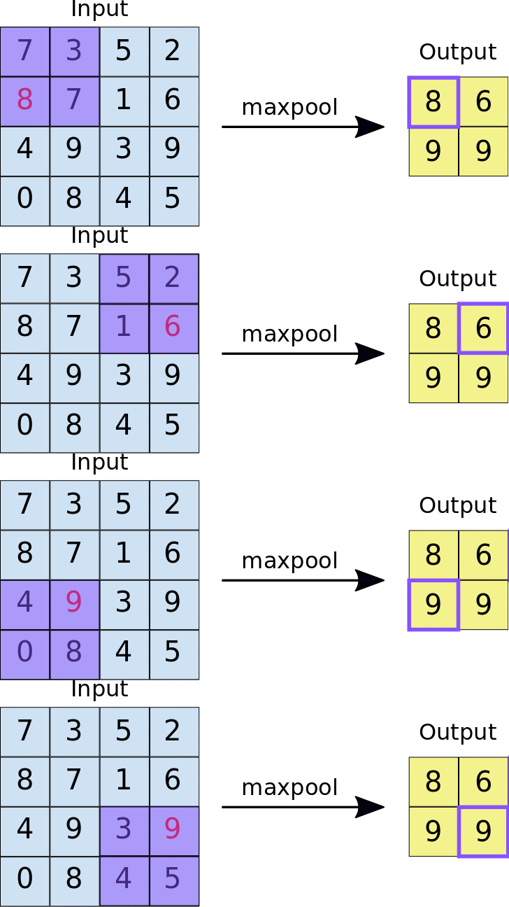
The second operation is performed using a pooling layer. The most common pooling layer is the max pooling. Similar to the convolution, the pooling is performed across the image. In the animation below, the pooling consists of a 2x2 pixel group converted into a single value using the maximum function.
Source: https://developers.google.com
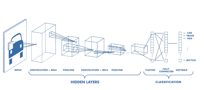
The network architecture shown below depicts a complete network. First the image goes through two sequence of convolution+pooling. The resulting image is then flatten and injected into a neural network.
Source: https://cdn-images-1.medium.com
# load data
mnist = tf.keras.datasets.mnist
(training_images, training_labels), (testing_images, testing_labels) = mnist.load_data()

training_images = np.expand_dims(training_images,4)
testing_images = np.expand_dims(testing_images,4)

# Shapes
print(training_images.shape)
print(training_labels.shape)
print(testing_images.shape)
print(testing_labels.shape)
(60000, 28, 28, 1)
(60000,)
(10000, 28, 28, 1)
(10000,)
# Import Image Generator
from tensorflow.keras.preprocessing.image import ImageDataGenerator

# Create an ImageDataGenerator and do Image Augmentation
train_datagen = ImageDataGenerator(
    rescale = 1/255.0
    )

validation_datagen = ImageDataGenerator(
    rescale = 1/255.0
    )
# create CNN Conv2D_64 -> MaxPooling_2 -> Conv2D_64 -> MaxPooling_2 -> NN_128 -> NN_10
model_cnn = tf.keras.models.Sequential([

    tf.keras.layers.Conv2D(32, (5,5), activation='relu', input_shape=(28, 28, 1), padding='same'),
    tf.keras.layers.MaxPooling2D(2, 2),
    tf.keras.layers.Dropout(0.25),

    tf.keras.layers.Conv2D(32, (5,5), activation='relu', padding='same'),
    tf.keras.layers.MaxPooling2D(2,2),
    tf.keras.layers.Dropout(0.25),

    tf.keras.layers.Flatten(),

    tf.keras.layers.Dense(256,activation='relu'),
    tf.keras.layers.Dropout(0.5),

    tf.keras.layers.Dense(10,activation='softmax')
])
The role of the optimizer is to adjust internal parameters (weights, bias,…) in order to help minimizing the loss.
# compile model
model_cnn.compile(
    optimizer = 'adam',
    loss = 'sparse_categorical_crossentropy',
    metrics = ['accuracy']
    )
Before training the model, we also implement a change into the learning rate. The learning rate of the model describes how fast the model moves toward a minimim. As the loss function gets closer to its minimum, we want the learning rate to slow down in order to improve the convergence.
We will keep a “large” initial learning rate to speed up the first iterations and the learning rate will be reduced during the training process.
# summary
model_cnn.summary()
Model: "sequential_2"
_________________________________________________________________
Layer (type)                 Output Shape              Param #
=================================================================
conv2d (Conv2D)              (None, 28, 28, 32)        832
_________________________________________________________________
max_pooling2d (MaxPooling2D) (None, 14, 14, 32)        0
_________________________________________________________________
dropout_3 (Dropout)          (None, 14, 14, 32)        0
_________________________________________________________________
conv2d_1 (Conv2D)            (None, 14, 14, 32)        25632
_________________________________________________________________
max_pooling2d_1 (MaxPooling2 (None, 7, 7, 32)          0
_________________________________________________________________
dropout_4 (Dropout)          (None, 7, 7, 32)          0
_________________________________________________________________
flatten_2 (Flatten)          (None, 1568)              0
_________________________________________________________________
dense_8 (Dense)              (None, 256)               401664
_________________________________________________________________
dropout_5 (Dropout)          (None, 256)               0
_________________________________________________________________
dense_9 (Dense)              (None, 10)                2570
=================================================================
Total params: 430,698
Trainable params: 430,698
Non-trainable params: 0
_________________________________________________________________
# Train the Model
history_no_augm = model_cnn.fit_generator(
    train_datagen.flow(training_images, training_labels, batch_size=32),
    steps_per_epoch=len(training_images) / 32,
    epochs=30,
    verbose=1,
    validation_data=validation_datagen.flow(testing_images, testing_labels, batch_size=32),
    validation_steps=len(testing_images) / 32)
Epoch 1/30
1875/1875 [==============================] - 88s 47ms/step - loss: 0.1924 - acc: 0.9391 - val_loss: 0.0425 - val_acc: 0.9855
Epoch 2/30
1875/1875 [==============================] - 76s 41ms/step - loss: 0.0738 - acc: 0.9778 - val_loss: 0.0296 - val_acc: 0.9904
Epoch 3/30
1875/1875 [==============================] - 70s 38ms/step - loss: 0.0575 - acc: 0.9827 - val_loss: 0.0249 - val_acc: 0.9905
Epoch 4/30
1875/1875 [==============================] - 70s 37ms/step - loss: 0.0503 - acc: 0.9846 - val_loss: 0.0234 - val_acc: 0.9921
Epoch 5/30
1875/1875 [==============================] - 70s 37ms/step - loss: 0.0440 - acc: 0.9864 - val_loss: 0.0225 - val_acc: 0.9920
Epoch 6/30
1875/1875 [==============================] - 70s 37ms/step - loss: 0.0397 - acc: 0.9877 - val_loss: 0.0208 - val_acc: 0.9927
Epoch 7/30
1875/1875 [==============================] - 70s 37ms/step - loss: 0.0361 - acc: 0.9892 - val_loss: 0.0194 - val_acc: 0.9932
Epoch 8/30
1875/1875 [==============================] - 70s 38ms/step - loss: 0.0325 - acc: 0.9898 - val_loss: 0.0221 - val_acc: 0.9919
Epoch 9/30
1875/1875 [==============================] - 70s 37ms/step - loss: 0.0317 - acc: 0.9899 - val_loss: 0.0215 - val_acc: 0.9926
Epoch 10/30
1875/1875 [==============================] - 73s 39ms/step - loss: 0.0296 - acc: 0.9904 - val_loss: 0.0184 - val_acc: 0.9939
Epoch 11/30
1875/1875 [==============================] - 73s 39ms/step - loss: 0.0281 - acc: 0.9917 - val_loss: 0.0181 - val_acc: 0.9944
Epoch 12/30
1875/1875 [==============================] - 70s 37ms/step - loss: 0.0281 - acc: 0.9914 - val_loss: 0.0216 - val_acc: 0.9930
Epoch 13/30
1875/1875 [==============================] - 70s 37ms/step - loss: 0.0280 - acc: 0.9916 - val_loss: 0.0196 - val_acc: 0.9936
Epoch 14/30
1875/1875 [==============================] - 70s 37ms/step - loss: 0.0240 - acc: 0.9923 - val_loss: 0.0201 - val_acc: 0.9937
Epoch 15/30
1875/1875 [==============================] - 70s 37ms/step - loss: 0.0234 - acc: 0.9928 - val_loss: 0.0188 - val_acc: 0.9942
Epoch 16/30
1875/1875 [==============================] - 69s 37ms/step - loss: 0.0250 - acc: 0.9927 - val_loss: 0.0175 - val_acc: 0.9943
Epoch 17/30
1875/1875 [==============================] - 69s 37ms/step - loss: 0.0222 - acc: 0.9928 - val_loss: 0.0168 - val_acc: 0.9946
Epoch 18/30
1875/1875 [==============================] - 70s 37ms/step - loss: 0.0227 - acc: 0.9930 - val_loss: 0.0212 - val_acc: 0.9937
Epoch 19/30
1875/1875 [==============================] - 69s 37ms/step - loss: 0.0222 - acc: 0.9934 - val_loss: 0.0209 - val_acc: 0.9935
Epoch 20/30
1875/1875 [==============================] - 69s 37ms/step - loss: 0.0245 - acc: 0.9927 - val_loss: 0.0183 - val_acc: 0.9949
Epoch 21/30
1875/1875 [==============================] - 70s 37ms/step - loss: 0.0225 - acc: 0.9934 - val_loss: 0.0201 - val_acc: 0.9946
Epoch 22/30
1875/1875 [==============================] - 69s 37ms/step - loss: 0.0227 - acc: 0.9933 - val_loss: 0.0187 - val_acc: 0.9943
Epoch 23/30
1875/1875 [==============================] - 70s 37ms/step - loss: 0.0198 - acc: 0.9940 - val_loss: 0.0189 - val_acc: 0.9948
Epoch 24/30
1875/1875 [==============================] - 71s 38ms/step - loss: 0.0212 - acc: 0.9937 - val_loss: 0.0214 - val_acc: 0.9946
Epoch 25/30
1875/1875 [==============================] - 70s 38ms/step - loss: 0.0224 - acc: 0.9929 - val_loss: 0.0196 - val_acc: 0.9951
Epoch 26/30
1875/1875 [==============================] - 69s 37ms/step - loss: 0.0214 - acc: 0.9936 - val_loss: 0.0199 - val_acc: 0.9947
Epoch 27/30
1875/1875 [==============================] - 69s 37ms/step - loss: 0.0195 - acc: 0.9941 - val_loss: 0.0211 - val_acc: 0.9945
Epoch 28/30
1875/1875 [==============================] - 79s 42ms/step - loss: 0.0206 - acc: 0.9939 - val_loss: 0.0189 - val_acc: 0.9948
Epoch 29/30
1875/1875 [==============================] - 79s 42ms/step - loss: 0.0207 - acc: 0.9941 - val_loss: 0.0193 - val_acc: 0.9952
Epoch 30/30
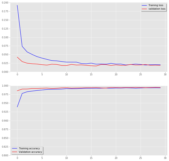
1875/1875 [==============================] - 83s 44ms/step - loss: 0.0205 - acc: 0.9939 - val_loss: 0.0188 - val_acc: 0.9950
# evaluate performance
print("Training = ")
model_cnn.evaluate(training_images/255.0, training_labels)

print("\nTest = ")
model_cnn.evaluate(testing_images/255.0, testing_labels)
Training =
60000/60000 [==============================] - 13s 209us/sample - loss: 0.0024 - acc: 0.9994

Test =
10000/10000 [==============================] - 2s 204us/sample - loss: 0.0188 - acc: 0.9950

[0.018755361672989995, 0.995]
# Plot the loss and accuracy curves for training and validation
fig, ax = plt.subplots(2,1,figsize=(12,12))
ax[0].plot(history_no_augm.history['loss'], color='b', label="Training loss")
ax[0].plot(history_no_augm.history['val_loss'], color='r', label="validation loss",axes =ax[0])
legend = ax[0].legend(loc='best', shadow=True)
ax[0].set_ylim(0,)

ax[1].plot(history_no_augm.history['acc'], color='b', label="Training accuracy")
ax[1].plot(history_no_augm.history['val_acc'], color='r',label="Validation accuracy")
legend = ax[1].legend(loc='best', shadow=True)
ax[1].set_ylim(0.8,1.0);
# Plot non-normalized confusion matrix
Y_test_pred = model_cnn.predict(testing_images/255.0)
Y_test_pred = Y_test_pred.argmax(axis=1)

TAD_tools.plot_confusion_matrix(testing_labels, Y_test_pred, classes=np.array([str(x) for x in range(11)]),
                     title='Confusion matrix, without normalization');

TAD_tools.plot_worst_predictions(model_cnn,testing_images/255.0,testing_labels)
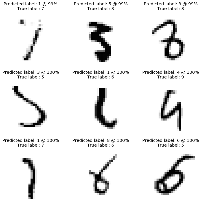
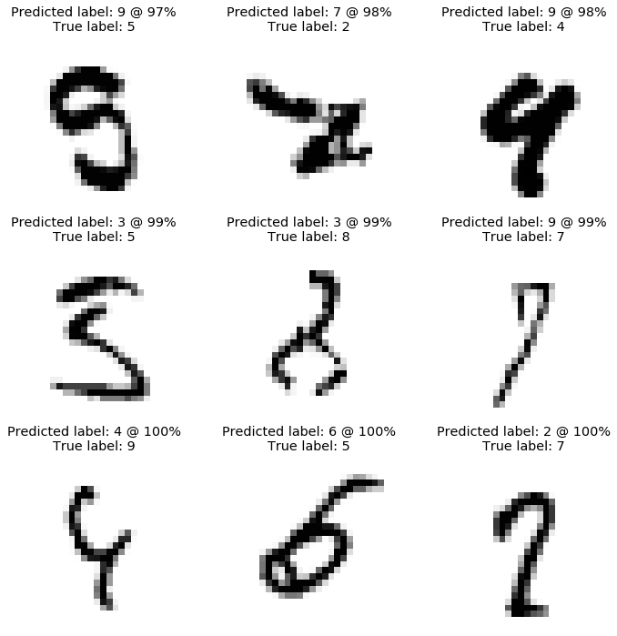
From the above, we can see that our model approaches human-prediction baseline. Indeed, several of these digits cannot be properly identified by a human eye.
TAD_tools.plot_convolutions_v2(model_cnn,testing_images/1.0)


df_results = df_results.append({'Model':"CNN",
                                'Training accuracy':history_no_augm.history['acc'][-1],
                                'Testing accuracy':history_no_augm.history['val_acc'][-1]},ignore_index=True)
5. Convolutional Networks (CNN) with data augmentation
# load data
mnist = tf.keras.datasets.mnist
(training_images, training_labels), (testing_images, testing_labels) = mnist.load_data()

training_images = np.expand_dims(training_images,4)
testing_images = np.expand_dims(testing_images,4)
# Import Image Generator
from tensorflow.keras.preprocessing.image import ImageDataGenerator

# Create an ImageDataGenerator and do Image Augmentation
train_datagen_augm = ImageDataGenerator(
    rescale = 1/255.0,
    zoom_range = 0.1,
    rotation_range = 10,
    width_shift_range = 0.1,
    height_shift_range = 0.1
    )

train_datagen.fit(training_images, augment=True)

validation_datagen = ImageDataGenerator(
    rescale = 1/255.0
    )
# create CNN Conv2D_64 -> MaxPooling_2 -> Conv2D_64 -> MaxPooling_2 -> NN_128 -> NN_10
model_cnn_augm = tf.keras.models.Sequential([

    tf.keras.layers.Conv2D(32, (5,5), activation='relu', input_shape=(28, 28, 1), padding='same'),
    tf.keras.layers.MaxPooling2D(2, 2),
    tf.keras.layers.Dropout(0.25),

    tf.keras.layers.Conv2D(32, (5,5), activation='relu', padding='same'),
    tf.keras.layers.MaxPooling2D(2,2),
    tf.keras.layers.Dropout(0.25),

    tf.keras.layers.Flatten(),

    tf.keras.layers.Dense(256,activation='relu'),
    tf.keras.layers.Dropout(0.5),

    tf.keras.layers.Dense(10,activation='softmax')
])
# compile model
model_cnn_augm.compile(
    optimizer = 'adam',
    loss = 'sparse_categorical_crossentropy',
    metrics = ['accuracy']
    )
model_cnn_augm.summary()
Model: "sequential_3"
_________________________________________________________________
Layer (type)                 Output Shape              Param #
=================================================================
conv2d_2 (Conv2D)            (None, 28, 28, 32)        832
_________________________________________________________________
max_pooling2d_2 (MaxPooling2 (None, 14, 14, 32)        0
_________________________________________________________________
dropout_6 (Dropout)          (None, 14, 14, 32)        0
_________________________________________________________________
conv2d_3 (Conv2D)            (None, 14, 14, 32)        25632
_________________________________________________________________
max_pooling2d_3 (MaxPooling2 (None, 7, 7, 32)          0
_________________________________________________________________
dropout_7 (Dropout)          (None, 7, 7, 32)          0
_________________________________________________________________
flatten_3 (Flatten)          (None, 1568)              0
_________________________________________________________________
dense_10 (Dense)             (None, 256)               401664
_________________________________________________________________
dropout_8 (Dropout)          (None, 256)               0
_________________________________________________________________
dense_11 (Dense)             (None, 10)                2570
=================================================================
Total params: 430,698
Trainable params: 430,698
Non-trainable params: 0
_________________________________________________________________
# Augmented training set
training_set = train_datagen_augm.flow(training_images, training_labels, batch_size=32)
validation_set = validation_datagen.flow(testing_images, testing_labels, batch_size=32)
# Train the Model
history_augm = model_cnn_augm.fit_generator(
    training_set,
    steps_per_epoch=len(training_images) / 32,
    epochs=30,
    verbose=1,
    validation_data=validation_set,
    validation_steps=len(testing_images) / 32)
Epoch 1/30
1875/1875 [==============================] - 81s 43ms/step - loss: 0.3100 - acc: 0.9015 - val_loss: 0.0379 - val_acc: 0.9862
Epoch 2/30
1875/1875 [==============================] - 78s 41ms/step - loss: 0.1261 - acc: 0.9620 - val_loss: 0.0286 - val_acc: 0.9888
Epoch 3/30
1875/1875 [==============================] - 74s 40ms/step - loss: 0.1016 - acc: 0.9700 - val_loss: 0.0247 - val_acc: 0.9917
Epoch 4/30
1875/1875 [==============================] - 78s 41ms/step - loss: 0.0865 - acc: 0.9740 - val_loss: 0.0222 - val_acc: 0.9929
Epoch 5/30
1875/1875 [==============================] - 76s 41ms/step - loss: 0.0794 - acc: 0.9752 - val_loss: 0.0210 - val_acc: 0.9928
Epoch 6/30
1875/1875 [==============================] - 84s 45ms/step - loss: 0.0747 - acc: 0.9769 - val_loss: 0.0191 - val_acc: 0.9931
Epoch 7/30
1875/1875 [==============================] - 82s 44ms/step - loss: 0.0703 - acc: 0.9795 - val_loss: 0.0171 - val_acc: 0.9945
Epoch 8/30
1875/1875 [==============================] - 95s 51ms/step - loss: 0.0638 - acc: 0.9808 - val_loss: 0.0194 - val_acc: 0.9936
Epoch 9/30
1875/1875 [==============================] - 79s 42ms/step - loss: 0.0660 - acc: 0.9801 - val_loss: 0.0193 - val_acc: 0.9933
Epoch 10/30
1875/1875 [==============================] - 76s 41ms/step - loss: 0.0621 - acc: 0.9815 - val_loss: 0.0171 - val_acc: 0.9944
Epoch 11/30
1875/1875 [==============================] - 80s 43ms/step - loss: 0.0612 - acc: 0.9822 - val_loss: 0.0173 - val_acc: 0.9944
Epoch 12/30
1875/1875 [==============================] - 81s 43ms/step - loss: 0.0580 - acc: 0.9825 - val_loss: 0.0174 - val_acc: 0.9940
Epoch 13/30
1875/1875 [==============================] - 74s 39ms/step - loss: 0.0564 - acc: 0.9830 - val_loss: 0.0189 - val_acc: 0.9942
Epoch 14/30
1875/1875 [==============================] - 74s 40ms/step - loss: 0.0571 - acc: 0.9830 - val_loss: 0.0217 - val_acc: 0.9928
Epoch 15/30
1875/1875 [==============================] - 78s 42ms/step - loss: 0.0559 - acc: 0.9834 - val_loss: 0.0193 - val_acc: 0.9937
Epoch 16/30
1875/1875 [==============================] - 75s 40ms/step - loss: 0.0561 - acc: 0.9837 - val_loss: 0.0185 - val_acc: 0.9937
Epoch 17/30
1875/1875 [==============================] - 74s 39ms/step - loss: 0.0542 - acc: 0.9840 - val_loss: 0.0205 - val_acc: 0.9925
Epoch 18/30
1875/1875 [==============================] - 77s 41ms/step - loss: 0.0529 - acc: 0.9842 - val_loss: 0.0184 - val_acc: 0.9939
Epoch 19/30
1875/1875 [==============================] - 78s 42ms/step - loss: 0.0555 - acc: 0.9839 - val_loss: 0.0194 - val_acc: 0.9943
Epoch 20/30
1875/1875 [==============================] - 78s 42ms/step - loss: 0.0539 - acc: 0.9839 - val_loss: 0.0190 - val_acc: 0.9943
Epoch 21/30
1875/1875 [==============================] - 78s 42ms/step - loss: 0.0540 - acc: 0.9845 - val_loss: 0.0217 - val_acc: 0.9924
Epoch 22/30
1875/1875 [==============================] - 77s 41ms/step - loss: 0.0521 - acc: 0.9851 - val_loss: 0.0196 - val_acc: 0.9938
Epoch 23/30
1875/1875 [==============================] - 92s 49ms/step - loss: 0.0542 - acc: 0.9849 - val_loss: 0.0191 - val_acc: 0.9939
Epoch 24/30
1875/1875 [==============================] - 82s 44ms/step - loss: 0.0496 - acc: 0.9851 - val_loss: 0.0225 - val_acc: 0.9935
Epoch 25/30
1875/1875 [==============================] - 86s 46ms/step - loss: 0.0526 - acc: 0.9843 - val_loss: 0.0220 - val_acc: 0.9940
Epoch 26/30
1875/1875 [==============================] - 82s 44ms/step - loss: 0.0479 - acc: 0.9862 - val_loss: 0.0210 - val_acc: 0.9937
Epoch 27/30
1875/1875 [==============================] - 79s 42ms/step - loss: 0.0493 - acc: 0.9858 - val_loss: 0.0204 - val_acc: 0.9933
Epoch 28/30
1875/1875 [==============================] - 78s 42ms/step - loss: 0.0510 - acc: 0.9857 - val_loss: 0.0190 - val_acc: 0.9941
Epoch 29/30
1875/1875 [==============================] - 91s 49ms/step - loss: 0.0511 - acc: 0.9854 - val_loss: 0.0191 - val_acc: 0.9942
Epoch 30/30
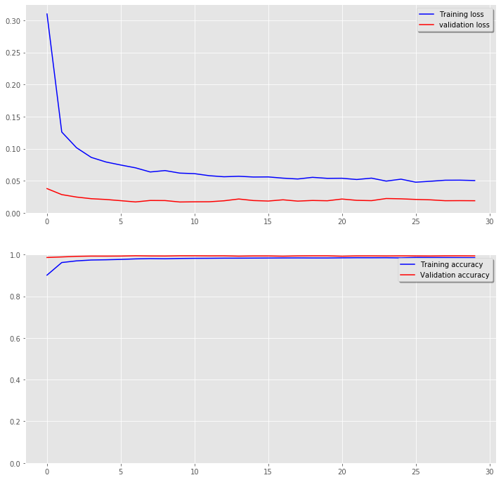
1875/1875 [==============================] - 86s 46ms/step - loss: 0.0505 - acc: 0.9851 - val_loss: 0.0190 - val_acc: 0.9938
# evaluate performance
print("Training = ")
model_cnn_augm.evaluate(training_images/255.0, training_labels)

print("\nTest = ")
model_cnn_augm.evaluate(testing_images/255.0, testing_labels)
Training =
60000/60000 [==============================] - 13s 212us/sample - loss: 0.0128 - acc: 0.9959

Test =
10000/10000 [==============================] - 2s 199us/sample - loss: 0.0190 - acc: 0.9938

[0.019008814232396254, 0.9938]
# Plot the loss and accuracy curves for training and validation
fig, ax = plt.subplots(2,1,figsize=(12,12))
ax[0].plot(history_augm.history['loss'], color='b', label="Training loss")
ax[0].plot(history_augm.history['val_loss'], color='r', label="validation loss",axes =ax[0])
legend = ax[0].legend(loc='best', shadow=True)
ax[0].set_ylim(0,)

ax[1].plot(history_augm.history['acc'], color='b', label="Training accuracy")
ax[1].plot(history_augm.history['val_acc'], color='r',label="Validation accuracy")
legend = ax[1].legend(loc='best', shadow=True)
ax[1].set_ylim(0.0,1.0);
# Plot non-normalized confusion matrix
Y_test_pred = model_cnn_augm.predict(testing_images/255.0)
Y_test_pred = Y_test_pred.argmax(axis=1)

TAD_tools.plot_confusion_matrix(testing_labels, Y_test_pred, classes=np.array([str(x) for x in range(11)]),
                     title='Confusion matrix, without normalization');
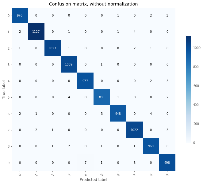
TAD_tools.plot_worst_predictions(model_cnn_augm,testing_images/255.0,testing_labels)
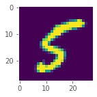
TAD_tools.plot_convolutions_v2(model_cnn_augm,testing_images/1.0)


df_results = df_results.append({'Model':"CNN Augmented",
                                'Training accuracy':history_augm.history['acc'][-1],
                                'Testing accuracy':history_augm.history['val_acc'][-1]},ignore_index=True)
6. Conclusion and Kaggle Submittal
As shown below, the best model correctly predicts the hand-written digits of the test set for 99.50% of the case (CCN no augmentation).
df_results
| Model | Training accuracy | Testing accuracy | |
|---|---|---|---|
| 0 | Log Reg | 0.911450 | 0.8987 |
| 1 | Lasso | 0.913900 | 0.9070 |
| 2 | Ridge | 0.920400 | 0.9152 |
| 3 | DNN No dropout | 0.997883 | 0.9786 |
| 4 | DNN Dropout | 0.990883 | 0.9829 |
| 5 | CNN | 0.993883 | 0.9950 |
| 6 | CNN Augmented | 0.985100 | 0.9938 |